Linear transformations, kernel and image

Vector spaces are the stage; linear transformations are the action. A linear transformation is a function between vector spaces that respects addition and scalar multiplication. In MATH-125 every linear transformation was multiplication by a matrix, \(\mathbf{x} \mapsto A\mathbf{x}\). Here the idea is broader: differentiation of polynomials, integration of functions, transposing a matrix, shifting a sequence and evaluating a polynomial at a point are all linear transformations, none of which starts life as a matrix. This lesson defines them, introduces the two subspaces that every linear map carries, the kernel and the image, and proves the rank–nullity theorem, which ties their dimensions together.

Definition and first examples

Let \(V\) and \(W\) be vector spaces. A function \(T : V \to W\) is a linear transformation (or linear map) if for all \(\mathbf{u}, \mathbf{v}\) in \(V\) and every scalar \(c\):

Equivalently, \(T(a\mathbf{u} + b\mathbf{v}) = aT(\mathbf{u}) + bT(\mathbf{v})\): \(T\) sends linear combinations to linear combinations with the same coefficients. Two consequences follow at once. \(T(\mathbf{0}) = \mathbf{0}\), because \(T(\mathbf{0}) = T(0\mathbf{0}) = 0T(\mathbf{0}) = \mathbf{0}\). And \(T\) is determined by what it does to a basis: if \(\mathbf{v} = c_1\mathbf{b}_1 + \dots + c_n\mathbf{b}_n\), then \(T(\mathbf{v}) = c_1T(\mathbf{b}_1) + \dots + c_nT(\mathbf{b}_n)\). Conversely, you may send the basis vectors anywhere you like, and there is exactly one linear map that does it.

A map \(V \to V\) from a space to itself is called a linear operator. Linear maps are everywhere:

• Differentiation \(D : P_3 \to P_2\), \(D(p) = p'\). The sum rule and the constant-multiple rule of calculus say exactly that \(D\) is linear.

• Integration \(J : C[0, 1] \to \mathbb{R}\), \(J(f) = \int_0^1 f(t)\,dt\).

• Evaluation \(E_2 : P_n \to \mathbb{R}\), \(E_2(p) = p(2)\).

• Transpose \(M_{m \times n} \to M_{n \times m}\), \(A \mapsto A^T\).

• The left shift on sequences, \((x_1, x_2, x_3, \dots) \mapsto (x_2, x_3, x_4, \dots)\).

• Rotations, reflections, projections and shears of the plane, which MATH-125 described with \(2 \times 2\) matrices.

Some familiar functions are not linear. Translation \(\mathbf{x} \mapsto \mathbf{x} + \mathbf{a}\) with \(\mathbf{a} \ne \mathbf{0}\) moves the origin, so it fails \(T(\mathbf{0}) = \mathbf{0}\). The determinant on \(M_{2 \times 2}\) is not linear, because \(\det(2A) = 4\det A\). The map \(p \mapsto p^2\) on polynomials is not linear. A quick test: check whether zero goes to zero, then try doubling an input.

The kernel

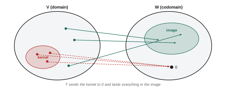
The kernel (or null space) of \(T : V \to W\) is the set of inputs that \(T\) sends to zero:

It is a subspace of \(V\): it contains \(\mathbf{0}\), and if \(T(\mathbf{u}) = T(\mathbf{v}) = \mathbf{0}\) then \(T(a\mathbf{u} + b\mathbf{v}) = \mathbf{0}\). For a matrix map \(\mathbf{x} \mapsto A\mathbf{x}\), the kernel is \(\operatorname{Nul} A\). For \(D : P_3 \to P_2\), the kernel is the constant polynomials, a one-dimensional subspace. For evaluation at 2 on \(P_n\), the kernel is the polynomials with a root at 2, which are the multiples of \(t - 2\).

The kernel measures how much information \(T\) destroys. Theorem: \(T\) is one-to-one (injective) if and only if \(\ker T = \{\mathbf{0}\}\). Proof: if \(T\) is one-to-one, only \(\mathbf{0}\) maps to \(\mathbf{0}\). Conversely, if the kernel is trivial and \(T(\mathbf{u}) = T(\mathbf{v})\), then \(T(\mathbf{u} - \mathbf{v}) = \mathbf{0}\), so \(\mathbf{u} - \mathbf{v} = \mathbf{0}\). This is far easier to check than the definition of one-to-one, because you only have to solve one equation, \(T(\mathbf{v}) = \mathbf{0}\).

The kernel also describes all solutions of a linear equation. If \(T(\mathbf{v}_p) = \mathbf{w}\), then the full solution set of \(T(\mathbf{v}) = \mathbf{w}\) is \(\mathbf{v}_p + \ker T\): one particular solution plus anything in the kernel. You saw this for \(A\mathbf{x} = \mathbf{b}\) in MATH-125; it holds equally for linear differential equations, where the general solution is a particular solution plus the general solution of the homogeneous equation.

The image

The image (or range) of \(T\) is the set of all outputs:

It is a subspace of \(W\), because sums and multiples of outputs are outputs of sums and multiples. If \(\mathbf{b}_1, \dots, \mathbf{b}_n\) is a basis of \(V\), then \(\operatorname{im} T = \operatorname{span}\{T(\mathbf{b}_1), \dots, T(\mathbf{b}_n)\}\). For a matrix map the image is the column space. \(T\) is onto (surjective) exactly when \(\operatorname{im} T = W\). The dimension of the image is called the rank of \(T\), and the dimension of the kernel its nullity.

The rank–nullity theorem

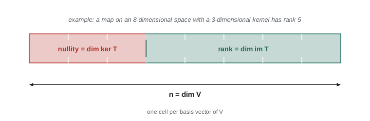
Theorem (rank–nullity). If \(V\) is finite-dimensional and \(T : V \to W\) is linear, then

Proof. Let \(\mathbf{k}_1, \dots, \mathbf{k}_r\) be a basis of \(\ker T\), and extend it to a basis \(\mathbf{k}_1, \dots, \mathbf{k}_r, \mathbf{v}_1, \dots, \mathbf{v}_s\) of \(V\), so \(\dim V = r + s\). We show that \(T(\mathbf{v}_1), \dots, T(\mathbf{v}_s)\) is a basis of the image, which gives \(\dim(\operatorname{im} T) = s\). Spanning: any output is \(T\) of a combination of the basis, and \(T\) kills the \(\mathbf{k}\)s, so it is a combination of the \(T(\mathbf{v}_j)\). Independence: if \(c_1T(\mathbf{v}_1) + \dots + c_sT(\mathbf{v}_s) = \mathbf{0}\), then \(T(c_1\mathbf{v}_1 + \dots + c_s\mathbf{v}_s) = \mathbf{0}\), so \(c_1\mathbf{v}_1 + \dots + c_s\mathbf{v}_s\) lies in the kernel and equals some combination of the \(\mathbf{k}\)s. Moving everything to one side gives a combination of the basis of \(V\) equal to zero, so all coefficients vanish; in particular every \(c_j = 0\).

Rank–nullity is a conservation law: every dimension of the input either survives into the image or is lost in the kernel. For \(D : P_3 \to P_2\), \(\dim P_3 = 4\), the kernel (constants) has dimension 1, so the image has dimension 3, which is all of \(P_2\): every polynomial of degree at most 2 is a derivative. For an \(m \times n\) matrix it reads \(n = \dim \operatorname{Nul} A + \operatorname{rank} A\), the count of free variables plus pivots you met in MATH-125.

Consequences

Rank–nullity answers existence and uniqueness questions without computation. If \(\dim V > \dim W\), then \(\operatorname{rank} T \le \dim W < \dim V\), so the nullity is positive and \(T\) cannot be one-to-one: a linear map cannot squeeze a bigger space into a smaller one without collapsing something. If \(\dim V < \dim W\), the image has dimension at most \(\dim V\), so \(T\) cannot be onto. If \(\dim V = \dim W\), then one-to-one and onto are equivalent: a trivial kernel forces a full-dimensional image, and vice versa.

That last fact has a striking application to interpolation. Given distinct numbers \(t_0, t_1, \dots, t_n\), consider \(T : P_n \to \mathbb{R}^{n+1}\), \(T(p) = (p(t_0), \dots, p(t_n))\). It is linear. Its kernel is the polynomials of degree at most \(n\) with \(n + 1\) distinct roots, and only the zero polynomial has that many, so the kernel is trivial. Both spaces have dimension \(n + 1\), so \(T\) is also onto: for any prescribed values \(y_0, \dots, y_n\) there is exactly one polynomial of degree at most \(n\) through the points \((t_i, y_i)\). We proved the existence of interpolating polynomials without constructing one.

Isomorphisms

A linear map that is both one-to-one and onto is an isomorphism, and two spaces are isomorphic, written \(V \cong W\), if there is an isomorphism between them. An isomorphism has a linear inverse, and it carries bases to bases, independent sets to independent sets and subspaces to subspaces of the same dimension. Isomorphic spaces are the same space in different clothing.

Theorem. Two finite-dimensional vector spaces are isomorphic if and only if they have the same dimension. Proof: an isomorphism sends a basis to a basis, so dimensions agree. Conversely, if both have dimension \(n\), the coordinate maps to \(\mathbb{R}^n\) are isomorphisms, and composing one with the inverse of the other gives \(V \cong W\).

So \(P_3\), \(M_{2 \times 2}\) and \(\mathbb{R}^4\) are all isomorphic. The theorem is the formal reason that choosing a basis lets you do all of linear algebra with columns of numbers. It does not mean the spaces are interchangeable for every purpose: \(P_3\) has multiplication of polynomials and \(M_{2 \times 2}\) has matrix multiplication, and those extra structures are not preserved by an arbitrary isomorphism. Linear algebra only sees the vector space structure.

Composition and the algebra of linear maps

If \(T : U \to V\) and \(S : V \to W\) are linear, the composition \(S \circ T : U \to W\), \((S \circ T)(\mathbf{u}) = S(T(\mathbf{u}))\), is linear. Sums \(S + T\) and multiples \(cT\) of linear maps between the same spaces are linear too, so the set of all linear maps from \(V\) to \(W\), written \(L(V, W)\), is itself a vector space. Composition corresponds to matrix multiplication, which explains why matrix multiplication is defined the way it is; lesson 4 makes this precise.

Composition gives useful rank inequalities. The image of \(S \circ T\) is contained in the image of \(S\), so \(\operatorname{rank}(S \circ T) \le \operatorname{rank} S\); and \(S \circ T\) can only lose dimensions from the image of \(T\), so \(\operatorname{rank}(S \circ T) \le \operatorname{rank} T\). For matrices, \(\operatorname{rank}(AB) \le \min(\operatorname{rank} A, \operatorname{rank} B)\).

Quotient spaces, briefly

Rank–nullity suggests that \(V\) is somehow 'kernel plus image'. Quotient spaces make that idea exact without choosing a complement. Given a subspace \(U\) of \(V\), declare two vectors equivalent if their difference lies in \(U\). The equivalence classes, called cosets \(\mathbf{v} + U\), form a vector space \(V/U\) with \((\mathbf{v} + U) + (\mathbf{w} + U) = (\mathbf{v} + \mathbf{w}) + U\) and \(c(\mathbf{v} + U) = c\mathbf{v} + U\). Geometrically, if \(U\) is a line through the origin in \(\mathbb{R}^3\), the cosets are all the lines parallel to it, and \(V/U\) is two-dimensional: \(\dim(V/U) = \dim V - \dim U\).

The first isomorphism theorem says that for any linear \(T : V \to W\), the map \(\mathbf{v} + \ker T \mapsto T(\mathbf{v})\) is an isomorphism from \(V / \ker T\) onto \(\operatorname{im} T\). Taking dimensions recovers rank–nullity. Quotients matter more in later algebra courses (MATH-322 builds group and ring quotients on the same pattern), so here we only need the picture: collapsing the kernel to a point leaves a copy of the image.

Computing kernel and image for the derivative

The code builds the matrix of \(D : P_3 \to P_2\) in the standard bases, then computes the rank and nullity exactly and checks rank–nullity. It also checks the second derivative \(D^2 : P_3 \to P_1\), whose kernel is the polynomials of degree at most 1.

from fractions import Fraction as F

def rank(rows):
    A = [[F(x) for x in r] for r in rows]
    m, n, r = len(A), len(A[0]), 0
    for c in range(n):
        p = next((i for i in range(r, m) if A[i][c] != 0), None)
        if p is None:
            continue
        A[r], A[p] = A[p], A[r]
        for i in range(r + 1, m):
            f = A[i][c] / A[r][c]
            A[i] = [a - f * b for a, b in zip(A[i], A[r])]
        r += 1
    return r

def derivative_matrix(n):
    """Matrix of D: P_n -> P_{n-1} in the bases 1, t, ..., t^n."""
    return [[(j if j == i + 1 else 0) for j in range(n + 1)] for i in range(n)]

D = derivative_matrix(3)
print("matrix of D: P3 -> P2")
for row in D:
    print("  ", row)
r = rank(D)
print("rank =", r, " nullity =", 4 - r, " dim P3 =", 4)

# second derivative: compose D (P3 -> P2) with D (P2 -> P1)
D2 = [[sum(derivative_matrix(2)[i][k] * D[k][j] for k in range(3)) for j in range(4)] for i in range(2)]
print("matrix of D^2: P3 -> P1:", D2)
r2 = rank(D2)
print("rank =", r2, " nullity =", 4 - r2, "(kernel: polynomials a + bt)")

matrix of D: P3 -> P2
   [0, 1, 0, 0]
   [0, 0, 2, 0]
   [0, 0, 0, 3]
rank = 3  nullity = 1  dim P3 = 4
matrix of D^2: P3 -> P1: [[0, 0, 2, 0], [0, 0, 0, 6]]
rank = 2  nullity = 2 (kernel: polynomials a + bt)

The matrix of \(D^2\) is the product of the two derivative matrices, illustrating that composition of maps is matrix multiplication. Its rank is 2 and its nullity is 2, matching the fact that \(p'' = 0\) exactly when \(p\) has degree at most 1.