
MATH-221 · Lesson 12 of 12 · 24 min
Capstone: the singular value decomposition and its applications
The spectral theorem gives symmetric matrices a perfect basis, orthonormal and made of eigenvectors. Most matrices are not symmetric, and many are not even square, yet every matrix has something almost as good. The singular value decomposition writes any \(m \times n\) matrix as a rotation, a stretch along the coordinate axes and another rotation, using two orthonormal bases, one for the domain and one for the codomain. It is the rank normal form of lesson 4 with orthonormal bases, it is built from the spectral theorem of lesson 11, and it solves the least squares problems of lesson 10 even when the columns are dependent. This capstone proves the SVD, reads the four fundamental subspaces off it, proves that truncating it gives the best low-rank approximation, and uses it for compression, the pseudoinverse, conditioning and principal component analysis.
Existence
Theorem (SVD). Let \(A\) be a real \(m \times n\) matrix of rank \(r\). There are orthogonal matrices \(U\) (\(m \times m\)) and \(V\) (\(n \times n\)) and numbers \(\sigma_1 \ge \sigma_2 \ge \dots \ge \sigma_r > 0\) such that
The \(\sigma_i\) are the singular values of \(A\); the columns \(\mathbf{v}_i\) of \(V\) and \(\mathbf{u}_i\) of \(U\) are the right and left singular vectors.
Proof. The matrix \(A^{T}A\) is symmetric and positive semidefinite, since \(\mathbf{x}^{T}A^{T}A\mathbf{x} = \|A\mathbf{x}\|^2 \ge 0\). By the spectral theorem it has an orthonormal eigenbasis \(\mathbf{v}_1, \dots, \mathbf{v}_n\) with eigenvalues \(\lambda_1 \ge \dots \ge \lambda_n \ge 0\). Its rank equals the rank of \(A\) (lesson 10 showed \(\ker A^{T}A = \ker A\)), so exactly \(r\) eigenvalues are positive. Set \(\sigma_i = \sqrt{\lambda_i}\) and, for \(i \le r\), \(\mathbf{u}_i = A\mathbf{v}_i/\sigma_i\). These are orthonormal:
Extend \(\mathbf{u}_1, \dots, \mathbf{u}_r\) to an orthonormal basis of \(\mathbb{R}^m\) (lesson 9). Then \(A\mathbf{v}_i = \sigma_i\mathbf{u}_i\) for \(i \le r\) and \(A\mathbf{v}_i = \mathbf{0}\) for \(i > r\), which is \(AV = U\Sigma\), that is, \(A = U\Sigma V^{T}\). The singular values are uniquely determined, being square roots of eigenvalues of \(A^{T}A\); the singular vectors are unique up to sign when the singular values are distinct.
Equivalently, the SVD is a sum of rank-one matrices, the outer product form
and keeping only the first \(r\) columns of \(U\) and \(V\) gives the compact SVD \(A = U_r\Sigma_rV_r^{T}\).
Geometry: rotate, stretch, rotate
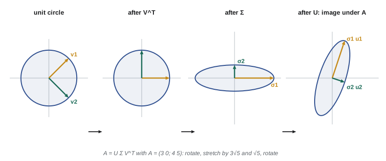
Read \(A\mathbf{x} = U\Sigma V^{T}\mathbf{x}\) from right to left. \(V^{T}\) is orthogonal, so it rotates (or reflects) the unit sphere to itself, carrying the \(\mathbf{v}_i\) to the standard axes. \(\Sigma\) stretches the \(i\)th axis by \(\sigma_i\), flattening the sphere into an ellipsoid and collapsing the last \(n - r\) axes. \(U\) rotates the result into position in \(\mathbb{R}^m\). So the image of the unit sphere under any matrix is an ellipsoid (possibly flattened) whose semi-axes are \(\sigma_i\mathbf{u}_i\). The largest singular value is the operator norm, \(\sigma_1 = \max_{\|\mathbf{x}\| = 1}\|A\mathbf{x}\|\), the greatest stretch, attained at \(\mathbf{v}_1\).
The four fundamental subspaces
The SVD gives orthonormal bases for all four fundamental subspaces at once:
| Subspace | Orthonormal basis from the SVD | Dimension |
|---|---|---|
| Column space \(\operatorname{im}A\) | \(\mathbf{u}_1, \dots, \mathbf{u}_r\) | \(r\) |
| Left null space \(\ker A^{T}\) | \(\mathbf{u}_{r+1}, \dots, \mathbf{u}_m\) | \(m - r\) |
| Row space \(\operatorname{im}A^{T}\) | \(\mathbf{v}_1, \dots, \mathbf{v}_r\) | \(r\) |
| Null space \(\ker A\) | \(\mathbf{v}_{r+1}, \dots, \mathbf{v}_n\) | \(n - r\) |
Restricted to the row space, \(A\) is an isomorphism onto the column space, sending the orthonormal basis \(\mathbf{v}_i\) to the orthogonal basis \(\sigma_i\mathbf{u}_i\). Everything else in the domain, the null space, is sent to zero. This is the complete geometric picture of a linear map between inner product spaces, and the rank in rank–nullity is simply the number of nonzero singular values. Numerically, the rank is decided by counting singular values above a tolerance, which is how numpy's matrix_rank works.
Best low-rank approximation
Truncating the outer product form after \(k\) terms gives \(A_k = \sigma_1\mathbf{u}_1\mathbf{v}_1^{T} + \dots + \sigma_k\mathbf{u}_k\mathbf{v}_k^{T}\), a matrix of rank \(k\).
Theorem (Eckart–Young–Mirsky). Among all matrices \(B\) of rank at most \(k\), \(A_k\) minimizes both the spectral norm and the Frobenius norm of \(A - B\), and
Proof for the spectral norm. The error \(A - A_k = \sum_{i>k}\sigma_i\mathbf{u}_i\mathbf{v}_i^{T}\) has largest singular value \(\sigma_{k+1}\). Now let \(B\) have rank at most \(k\). Its null space has dimension at least \(n - k\), and the span \(W\) of \(\mathbf{v}_1, \dots, \mathbf{v}_{k+1}\) has dimension \(k + 1\), so by the dimension formula of lesson 2 they meet in a nonzero vector; take a unit vector \(\mathbf{x}\) there. Then \((A - B)\mathbf{x} = A\mathbf{x} = \sum_{i \le k+1}\sigma_i(\mathbf{v}_i^{T}\mathbf{x})\mathbf{u}_i\), whose norm squared is \(\sum_{i \le k+1}\sigma_i^2(\mathbf{v}_i^{T}\mathbf{x})^2 \ge \sigma_{k+1}^2\). So \(\|A - B\|_2 \ge \sigma_{k+1}\). The Frobenius case uses a similar argument applied singular value by singular value.
This theorem is the mathematical basis of a great deal of data compression and denoising. An image stored as an \(m \times n\) matrix of gray levels needs \(mn\) numbers; its rank-\(k\) approximation needs \(k(m + n + 1)\). When the singular values decay quickly, a small \(k\) captures most of the image. The same idea underlies latent semantic analysis of documents, recommender systems built by low-rank matrix completion, and the low-rank adapters used to fine-tune large neural networks.
The pseudoinverse and least squares
Define the Moore–Penrose pseudoinverse by inverting the nonzero singular values: \(A^{+} = V\Sigma^{+}U^{T}\), where \(\Sigma^{+}\) is \(n \times m\) with \(1/\sigma_1, \dots, 1/\sigma_r\) on its diagonal. Then \(\hat{\mathbf{x}} = A^{+}\mathbf{b}\) is the least squares solution of \(A\mathbf{x} = \mathbf{b}\) with the smallest norm. Proof sketch: in the coordinates \(\mathbf{y} = V^{T}\mathbf{x}\) and \(\mathbf{c} = U^{T}\mathbf{b}\), orthogonality preserves norms and the problem becomes minimizing \(\sum_{i \le r}(\sigma_iy_i - c_i)^2 + \sum_{i > r}c_i^2\). The first sum is zero exactly when \(y_i = c_i/\sigma_i\) for \(i \le r\); the remaining \(y_i\) are free and the norm is smallest when they are zero.
When \(A\) has independent columns, \(A^{+} = (A^{T}A)^{-1}A^{T}\), recovering lesson 10; when \(A\) is invertible, \(A^{+} = A^{-1}\). In general \(AA^{+}\) is the orthogonal projection onto the column space and \(A^{+}A\) the projection onto the row space. Small singular values cause trouble: \(1/\sigma_i\) is huge, and noise in \(c_i\) is amplified. Truncated SVD discards singular values below a threshold; ridge regression replaces \(1/\sigma_i\) by \(\sigma_i/(\sigma_i^2 + \lambda)\), smoothly damping the small ones. Both are standard forms of regularization.
Conditioning
For a square invertible matrix, the condition number is \(\kappa(A) = \|A\|_2\|A^{-1}\|_2 = \sigma_1/\sigma_n\), and for a rectangular matrix of full column rank it is \(\sigma_1/\sigma_n\) as well. It bounds the relative change in the solution of \(A\mathbf{x} = \mathbf{b}\) caused by a relative change in \(\mathbf{b}\): \(\|\delta\mathbf{x}\|/\|\mathbf{x}\| \le \kappa(A)\|\delta\mathbf{b}\|/\|\mathbf{b}\|\). Geometrically, \(\kappa\) is the ratio of the longest to the shortest axis of the ellipsoid image of the unit sphere. Orthogonal matrices have \(\kappa = 1\), which is why the orthogonal methods of lessons 9 to 11 are so stable, and lesson 10's warning that \(\kappa(A^{T}A) = \kappa(A)^2\) is now immediate, since the singular values of \(A^{T}A\) are the \(\sigma_i^2\). A rule of thumb: with \(\kappa \approx 10^k\), expect to lose about \(k\) of the 16 decimal digits of double precision.
Principal component analysis
Let \(X\) be an \(n \times p\) data matrix with centered columns (each variable has mean zero). The sample covariance matrix is \(C = X^{T}X/(n - 1)\). If \(X = U\Sigma V^{T}\), then \(C = V\frac{\Sigma^{T}\Sigma}{n - 1}V^{T}\), so the right singular vectors of \(X\) are the eigenvectors of \(C\), the principal directions, and the variances along them are \(\sigma_i^2/(n - 1)\). The scores \(XV = U\Sigma\) are the coordinates of the data in the principal axes. Computing PCA from the SVD of \(X\), rather than the eigenvectors of \(C\), avoids forming \(X^{T}X\) and its squared condition number. By Eckart–Young, projecting the data onto the first \(k\) principal directions gives the best \(k\)-dimensional linear summary in the least squares sense. This is the PCA of AI-210, the shape analysis of point clouds in CMPUT-411, and the subspace methods for recognizing faces and objects in CMPUT-367.
Worked problem
The SVD of a small matrix
Find the singular values of \(A = \begin{pmatrix} 3 & 0 \\ 4 & 5 \end{pmatrix}\), its condition number, and the error of its best rank-one approximation.
Show solution
- \(A^{T}A = \begin{pmatrix} 25 & 20 \\ 20 & 25 \end{pmatrix}\), with eigenvalues \(45\) and \(5\) and eigenvectors \((1, 1)/\sqrt2\) and \((1, -1)/\sqrt2\).
- So \(\sigma_1 = \sqrt{45} = 3\sqrt5\) and \(\sigma_2 = \sqrt5\). Check: \(\sigma_1\sigma_2 = 15 = |\det A|\).
- \(\mathbf{u}_1 = A\mathbf{v}_1/\sigma_1 = (3, 9)/(\sqrt2 \cdot 3\sqrt5) = (1, 3)/\sqrt{10}\), and \(\mathbf{u}_2 = A\mathbf{v}_2/\sigma_2 = (3, -1)/\sqrt{10}\).
- \(\kappa(A) = \sigma_1/\sigma_2 = 3\), and the best rank-one approximation \(\sigma_1\mathbf{u}_1\mathbf{v}_1^{T}\) has spectral error \(\sigma_2 = \sqrt5\).
Answer: \(\sigma_1 = 3\sqrt5\), \(\sigma_2 = \sqrt5\), \(\kappa = 3\), and \(\|A - A_1\|_2 = \sqrt5\).
Computing with the SVD
The code builds a synthetic grayscale image with a few smooth features plus noise, compresses it with truncated SVDs, and checks the Eckart–Young error formula exactly. It then solves a rank-deficient least squares problem with the pseudoinverse and shows how a tiny singular value inflates the condition number.
import numpy as np
rng = np.random.default_rng(221)

# a 120 x 160 "image": smooth blobs and stripes plus a little noise
y, x = np.mgrid[0:120, 0:160] / 40.0
img = np.exp(-((x - 1.5) ** 2 + (y - 1.2) ** 2)) + 0.5 * np.sin(3 * x) * np.cos(2 * y) + 0.3 * (y > 1.5)
img += 0.02 * rng.standard_normal(img.shape)

U, s, Vt = np.linalg.svd(img, full_matrices=False)
print("leading singular values:", np.round(s[:6], 3))
for k in (1, 3, 5, 10, 20):
    Ak = (U[:, :k] * s[:k]) @ Vt[:k]
    err2 = np.linalg.norm(img - Ak, 2)
    errF = np.linalg.norm(img - Ak)
    storage = k * (img.shape[0] + img.shape[1] + 1) / img.size
    print(f"k={k:2d}: ||A-A_k||_2={err2:.4f} (sigma_k+1={s[k]:.4f})  "
          f"rel F error={errF / np.linalg.norm(img):.4f}  storage {100 * storage:.1f}%")

# minimum-norm least squares for a rank-deficient matrix
A = np.array([[1.0, 2.0, 3.0], [2.0, 4.0, 6.0], [1.0, 0.0, 1.0], [0.0, 1.0, 1.0]])
b = np.array([1.0, 2.0, 0.0, 1.0])
print("rank of A:", np.linalg.matrix_rank(A))
xp = np.linalg.pinv(A) @ b
print("pseudoinverse solution:", np.round(xp, 4), " norm", round(np.linalg.norm(xp), 4))
null = np.linalg.svd(A)[2][-1]
other = xp + 0.5 * null
print("another least squares solution has the same residual:",
      np.isclose(np.linalg.norm(A @ other - b), np.linalg.norm(A @ xp - b)), "but norm", round(np.linalg.norm(other), 4))

# condition number from singular values
for eps in (1e-1, 1e-4, 1e-8):
    M = np.array([[1.0, 1.0], [1.0, 1.0 + eps]])
    sv = np.linalg.svd(M, compute_uv=False)
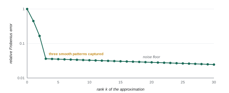
print(f"eps={eps:.0e}: sigma = {sv[0]:.4f}, {sv[1]:.2e} cond = {sv[0] / sv[1]:.2e}")leading singular values: [67.061 31.339 12.129 0.45 0.447 0.441] k= 1: ||A-A_k||_2=31.3390 (sigma_k+1=31.3390) rel F error=0.4492 storage 1.5% k= 3: ||A-A_k||_2=0.4499 (sigma_k+1=0.4499) rel F error=0.0361 storage 4.4% k= 5: ||A-A_k||_2=0.4411 (sigma_k+1=0.4411) rel F error=0.0351 storage 7.3% k=10: ||A-A_k||_2=0.4107 (sigma_k+1=0.4107) rel F error=0.0327 storage 14.6% k=20: ||A-A_k||_2=0.3541 (sigma_k+1=0.3541) rel F error=0.0284 storage 29.3% rank of A: 2 pseudoinverse solution: [-0.3333 0.4744 0.141 ] norm 0.5967 another least squares solution has the same residual: True but norm 0.7785 eps=1e-01: sigma = 2.0512, 4.88e-02 cond = 4.21e+01 eps=1e-04: sigma = 2.0001, 5.00e-05 cond = 4.00e+04 eps=1e-08: sigma = 2.0000, 5.00e-09 cond = 4.00e+08
The spectral-norm error of every truncation equals the next singular value, exactly as Eckart–Young predicts. Because the image is built from a few smooth patterns, the singular values fall off sharply and a handful of terms reproduce it closely while storing a small fraction of the numbers; beyond that, the remaining singular values mostly describe noise, so truncation also denoises. In the least squares example, adding a null-space vector leaves the residual unchanged but increases the norm, which is why the pseudoinverse solution is singled out. The last lines show the condition number growing like \(4/\varepsilon\) as the two rows become nearly parallel.
Looking back over the course
The singular value decomposition draws on almost every lesson. Vector spaces, bases and dimension (lessons 1 and 2) give the setting and the dimension count in the Eckart–Young proof. Linear maps, kernels and images (lesson 3) become the four fundamental subspaces. Change of basis (lesson 4) is the reason \(A = U\Sigma V^{T}\) is the same map in better coordinates. Eigenvalues and the spectral theorem (lessons 5, 6 and 11) produce the singular values. Inner products, orthogonality, projections and QR (lessons 9 and 10) make the bases orthonormal and the computations stable. Only the Jordan form (lessons 7 and 8) is absent, and its absence is itself a lesson: by insisting on orthonormal bases on both sides, the SVD trades the delicate, discontinuous structure of eigenvectors for a decomposition that always exists, is stable to compute and has a clear geometric meaning. That is why it is the workhorse of numerical linear algebra and data science.
Common mistakes
MistakeTaking the singular values to be the absolute values of the eigenvalues.
InsteadThat holds for symmetric (indeed normal) matrices; in general use the square roots of the eigenvalues of \(A^{T}A\).
MistakeComputing \(\mathbf{u}_i\) and \(\mathbf{v}_i\) as independent eigenvector problems for \(AA^{T}\) and \(A^{T}A\).
InsteadSigns must match; compute \(\mathbf{v}_i\) and then set \(\mathbf{u}_i = A\mathbf{v}_i/\sigma_i\).
MistakeInverting tiny singular values in the pseudoinverse without a threshold.
InsteadTruncate or regularize; tiny \(\sigma_i\) amplify noise.
MistakeRunning PCA on data whose columns have not been centered.
InsteadSubtract the column means first; otherwise the first component mostly points at the mean.
MistakeThinking the rank-k approximation keeps k rows or columns of the matrix.
InsteadIt is a sum of k rank-one matrices built from singular vectors; it generally changes every entry.
Summary and key terms
- Every real matrix factors as \(A = U\Sigma V^{T}\) with orthogonal \(U, V\) and non-negative singular values on the diagonal of \(\Sigma\).
- The singular values are the square roots of the eigenvalues of \(A^{T}A\); \(A\mathbf{v}_i = \sigma_i\mathbf{u}_i\).
- Geometrically, \(A\) rotates, stretches along axes and rotates; the unit sphere maps to an ellipsoid.
- The SVD gives orthonormal bases of the four fundamental subspaces, and the rank is the number of nonzero singular values.
- Truncating the SVD gives the best rank-\(k\) approximation, with spectral error \(\sigma_{k+1}\).
- The pseudoinverse gives the minimum-norm least squares solution; \(\kappa = \sigma_1/\sigma_n\) measures sensitivity.
- PCA is the SVD of a centered data matrix.
- singular value decomposition
- A factorization \(A = U\Sigma V^{T}\) with orthogonal \(U, V\) and diagonal non-negative \(\Sigma\).
- singular value
- A square root of an eigenvalue of \(A^{T}A\).
- singular vectors
- The orthonormal columns of \(U\) and \(V\).
- Eckart–Young theorem
- The truncated SVD is the best low-rank approximation in the spectral and Frobenius norms.
- pseudoinverse
- \(A^{+} = V\Sigma^{+}U^{T}\).
- operator norm
- The maximum of \(\|A\mathbf{x}\|\) over unit vectors, equal to \(\sigma_1\).
- condition number
- \(\sigma_1/\sigma_n\) for a matrix of full column rank.
- principal components
- The right singular vectors of a centered data matrix.
Practice problems
Work each problem on paper first, then reveal the answer to check.
Find the singular values of \(\begin{pmatrix} 1 & 1 \\ 0 & 0 \end{pmatrix}\).
Show answer
\(A^{T}A\) has eigenvalues 2 and 0, so \(\sigma_1 = \sqrt2\), \(\sigma_2 = 0\).
Prove that the singular values of an orthogonal matrix are all 1.
Show answer
\(Q^{T}Q = I\) has every eigenvalue 1.
Prove that \(\|A\|_2 = \sigma_1\).
Show answer
\(\|A\mathbf{x}\|^2 = \sum\sigma_i^2(\mathbf{v}_i^{T}\mathbf{x})^2 \le \sigma_1^2\|\mathbf{x}\|^2\), with equality at \(\mathbf{v}_1\).
Prove that \(|\det A| = \sigma_1\cdots\sigma_n\) for square \(A\).
Show answer
\(\det A = \det U \det\Sigma\det V^{T}\), and orthogonal determinants are \(\pm1\).
Show that \(AA^{+}\) is the orthogonal projection onto the column space.
Show answer
\(AA^{+} = U\Sigma\Sigma^{+}U^{T} = U_rU_r^{T}\).
For a symmetric positive semidefinite matrix, how do the SVD and the spectral decomposition compare?
Show answer
They coincide: \(U = V = Q\) and \(\Sigma = D\).
Lesson quiz · 5 questions
Score 60% or more to complete this lesson.
Create a free account to save your progress, take quizzes and earn a certificate.