
MATH-221 · Lesson 1 of 12 · 25 min
Vector spaces and subspaces
In MATH-125 you met vectors as arrows and as columns of numbers in \(\mathbb{R}^n\), and you learned to solve systems, multiply matrices, compute determinants and find eigenvalues. This course takes the next step. Instead of asking what we can do with columns of numbers, we ask what it is about columns of numbers that makes all of that work. The answer turns out to be a short list of rules, the vector space axioms, and once you see them you find vector spaces everywhere: in polynomials, in functions, in matrices, in sound signals, in solutions of differential equations, in sequences and in the pixels of an image.
Working at this level of generality pays off in two ways. First, one theorem proved for an abstract vector space applies at once to every example, so you prove things once and use them a hundred times. Second, the abstraction lets us see structure that coordinates hide. The derivative is a linear map on polynomials; least squares is a projection in a space of functions; the singular value decomposition, which ends this course, is a statement about any linear map between inner product spaces. Along the way the course becomes more proof-based than MATH-125. Each lesson includes short proofs to read and practice problems that ask you to write your own.
The axioms
A vector space over the real numbers is a set \(V\) of objects, called vectors, together with two operations: addition, which combines two vectors \(\mathbf{u}\) and \(\mathbf{v}\) into a vector \(\mathbf{u} + \mathbf{v}\), and scalar multiplication, which combines a real number \(c\) and a vector \(\mathbf{v}\) into a vector \(c\mathbf{v}\). The operations must satisfy ten axioms. For all \(\mathbf{u}, \mathbf{v}, \mathbf{w}\) in \(V\) and all real numbers \(a, b\):
- Closure under addition: \(\mathbf{u} + \mathbf{v}\) is in \(V\).
- Commutativity: \(\mathbf{u} + \mathbf{v} = \mathbf{v} + \mathbf{u}\).
- Associativity of addition: \((\mathbf{u} + \mathbf{v}) + \mathbf{w} = \mathbf{u} + (\mathbf{v} + \mathbf{w})\).
- Zero vector: there is a vector \(\mathbf{0}\) in \(V\) with \(\mathbf{v} + \mathbf{0} = \mathbf{v}\) for every \(\mathbf{v}\).
- Additive inverses: for each \(\mathbf{v}\) there is a vector \(-\mathbf{v}\) with \(\mathbf{v} + (-\mathbf{v}) = \mathbf{0}\).
- Closure under scalar multiplication: \(c\mathbf{v}\) is in \(V\).
- Distributivity over vector addition: \(a(\mathbf{u} + \mathbf{v}) = a\mathbf{u} + a\mathbf{v}\).
- Distributivity over scalar addition: \((a + b)\mathbf{v} = a\mathbf{v} + b\mathbf{v}\).
- Compatibility: \(a(b\mathbf{v}) = (ab)\mathbf{v}\).
- Identity: \(1\mathbf{v} = \mathbf{v}\).
Nothing in the list says what vectors are. They can be arrows, lists, functions or matrices. All that matters is that the two operations behave like the familiar ones. The real numbers used for scaling are called scalars. Replacing \(\mathbb{R}\) by the complex numbers \(\mathbb{C}\) gives a complex vector space, which we need in lessons 8 and 11 when eigenvalues turn out to be complex. Mathematicians also use other fields of scalars, such as the integers modulo a prime in coding theory, but in this course the scalars are real unless we say otherwise.
Consequences you can prove
The axioms are deliberately minimal. Familiar facts such as \(0\mathbf{v} = \mathbf{0}\) are not on the list; they follow from it. Proving them is good practice in using only what you are allowed to use.
Claim: for every vector \(\mathbf{v}\), \(0\mathbf{v} = \mathbf{0}\). Proof: by distributivity over scalar addition, \(0\mathbf{v} = (0 + 0)\mathbf{v} = 0\mathbf{v} + 0\mathbf{v}\). Add the additive inverse \(-(0\mathbf{v})\) to both sides. The left side becomes \(\mathbf{0}\); the right side becomes \(0\mathbf{v} + \mathbf{0} = 0\mathbf{v}\) after using associativity and the inverse and zero axioms. Hence \(0\mathbf{v} = \mathbf{0}\).
Similar short arguments show that the zero vector is unique, that each vector has exactly one additive inverse, that \(c\mathbf{0} = \mathbf{0}\) for every scalar \(c\), and that \((-1)\mathbf{v} = -\mathbf{v}\). The last fact is worth noticing: the additive inverse, defined abstractly by an axiom, turns out to be what you get by scaling by \(-1\). You will prove some of these in the practice questions.
Examples
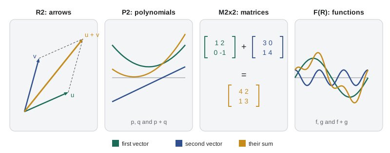
The point of the axioms is that many different objects satisfy them. Here are the examples we use throughout the course.
Euclidean space \(\mathbb{R}^n\). Vectors are ordered lists of \(n\) real numbers, added and scaled entry by entry. This is the model that MATH-125 studied.
Polynomials. \(P_n\) is the set of polynomials of degree at most \(n\) with real coefficients, such as \(p(t) = 3 - t + 4t^2\) in \(P_2\). Add polynomials by adding coefficients and scale by multiplying every coefficient. The zero vector is the zero polynomial. The set \(P\) of all polynomials, of any degree, is also a vector space.
Matrices. \(M_{m \times n}\) is the set of all \(m \times n\) real matrices, with the usual entrywise addition and scaling. The zero vector is the zero matrix.
Functions. \(F(\mathbb{R})\) is the set of all functions from \(\mathbb{R}\) to \(\mathbb{R}\), with \((f + g)(t) = f(t) + g(t)\) and \((cf)(t) = c\,f(t)\). The zero vector is the function that is zero everywhere. Inside it sit many smaller spaces: the continuous functions \(C(\mathbb{R})\), the differentiable functions, the functions on an interval such as \(C[0, 1]\).
Sequences. The set of all infinite sequences \((x_1, x_2, x_3, \dots)\) of real numbers, added and scaled term by term. Sequences appear in lesson 6 when we study recurrences like the Fibonacci numbers.
Solution sets. The set of all solutions of the homogeneous system \(A\mathbf{x} = \mathbf{0}\), and the set of all solutions of a linear homogeneous differential equation such as \(y'' + y = 0\), are vector spaces. That is why a general solution can be written as a combination of a few basic solutions.
| Space | A typical vector | Zero vector | Addition |
|---|---|---|---|
| \(\mathbb{R}^3\) | \((2, -1, 5)\) | \((0, 0, 0)\) | Entry by entry |
| \(P_2\) | \(3 - t + 4t^2\) | The zero polynomial | Add matching coefficients |
| \(M_{2 \times 2}\) | \(\begin{pmatrix} 1 & 2 \\ 0 & -3 \end{pmatrix}\) | The zero matrix | Entry by entry |
| \(C[0, 1]\) | \(f(t) = e^t\) | The function 0 | \((f + g)(t) = f(t) + g(t)\) |
| Sequences | \((1, 1, 2, 3, 5, \dots)\) | \((0, 0, 0, \dots)\) | Term by term |
Sets that are not vector spaces
Seeing what fails is as instructive as seeing what works. The set of polynomials of degree exactly 2 is not a vector space: \(t^2 + t\) and \(-t^2\) each have degree 2, but their sum \(t\) does not, so closure under addition fails, and the zero polynomial is missing. The first quadrant of the plane, \(\{(x, y) : x \ge 0, y \ge 0\}\), is closed under addition but not under multiplication by \(-1\). The line \(y = 2x + 1\) does not contain the origin, so it has no zero vector. The set of invertible \(2 \times 2\) matrices fails because the zero matrix is not invertible, and because the sum of two invertible matrices, such as \(I\) and \(-I\), can be singular.
Sometimes a set fails because the operations are unusual. Take \(\mathbb{R}^2\) with ordinary addition but with scalar multiplication defined as \(c(x, y) = (cx, 0)\). Every axiom holds except the identity axiom, because \(1(x, y) = (x, 0)\), which differs from \((x, y)\) whenever \(y \ne 0\). This shows why the identity axiom is on the list: without it, scaling could quietly throw information away.
Subspaces
Most of the vector spaces you meet in practice live inside a larger one. A subspace of a vector space \(V\) is a subset \(W\) that is itself a vector space using the same addition and scalar multiplication. Checking all ten axioms would be tedious, but most of them, such as commutativity, are inherited automatically from \(V\). Only closure and the presence of zero need checking.
Subspace test. A subset \(W\) of \(V\) is a subspace if and only if (1) \(W\) contains the zero vector of \(V\); (2) whenever \(\mathbf{u}\) and \(\mathbf{v}\) are in \(W\), so is \(\mathbf{u} + \mathbf{v}\); and (3) whenever \(\mathbf{v}\) is in \(W\) and \(c\) is a scalar, \(c\mathbf{v}\) is in \(W\). Conditions (2) and (3) are often combined into one: \(a\mathbf{u} + b\mathbf{v}\) is in \(W\) for all \(\mathbf{u}, \mathbf{v}\) in \(W\) and all scalars \(a, b\).
Why is this enough? Additive inverses come for free from condition (3), because \(-\mathbf{v} = (-1)\mathbf{v}\), which we proved above. All the identities among vectors hold in \(W\) because they hold in \(V\). Condition (1) could be replaced by 'W is non-empty', since if \(\mathbf{v}\) is in \(W\) then \(0\mathbf{v} = \mathbf{0}\) is too; but checking for zero first is the quickest way to rule out impostors such as lines that miss the origin.
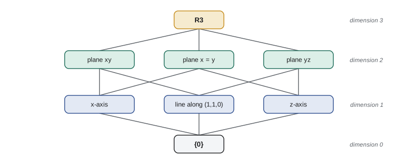
Every vector space has two trivial subspaces: \(\{\mathbf{0}\}\) and \(V\) itself. In \(\mathbb{R}^3\) the other subspaces are exactly the lines and planes through the origin, a fact we will prove once we have the idea of dimension in lesson 2.
Important families of subspaces
The null space of an \(m \times n\) matrix \(A\), written \(\operatorname{Nul} A\), is the set of all \(\mathbf{x}\) in \(\mathbb{R}^n\) with \(A\mathbf{x} = \mathbf{0}\). It is a subspace: \(A\mathbf{0} = \mathbf{0}\), and if \(A\mathbf{u} = \mathbf{0}\) and \(A\mathbf{v} = \mathbf{0}\) then \(A(a\mathbf{u} + b\mathbf{v}) = aA\mathbf{u} + bA\mathbf{v} = \mathbf{0}\). The column space \(\operatorname{Col} A\), the set of all combinations of the columns of \(A\), is a subspace of \(\mathbb{R}^m\). You met both in MATH-125; here they become examples of a general pattern.
In function spaces: the polynomials \(P_n\) form a subspace of \(C(\mathbb{R})\); the functions with \(f(0) = 0\) form a subspace; the even functions, with \(f(-t) = f(t)\), form a subspace; the solutions of \(y'' + y = 0\) form a subspace. In matrix spaces: the symmetric matrices (\(A^T = A\)), the upper triangular matrices, the diagonal matrices and the matrices with trace zero are all subspaces of \(M_{n \times n}\). The matrices with determinant zero are not, because determinant is not additive: \(\operatorname{diag}(1, 0)\) and \(\operatorname{diag}(0, 1)\) are both singular but their sum is \(I\).
Worked problem
Testing two subsets of the 2 by 2 matrices
Decide whether each set is a subspace of \(M_{2 \times 2}\): (a) the matrices with trace zero, \(a_{11} + a_{22} = 0\); (b) the matrices whose entries are all non-negative.
Show solution
- (a) Zero: the zero matrix has trace 0, so it belongs.
- (a) Closure: trace is additive and scales, \(\operatorname{tr}(aA + bB) = a\operatorname{tr}A + b\operatorname{tr}B\). If both traces are 0, so is the trace of the combination. So (a) is a subspace.
- (b) Zero: the zero matrix has all entries non-negative, so the first condition holds.
- (b) Scaling: the identity matrix is in the set, but \((-1)I\) has negative entries. Closure under scalar multiplication fails, so (b) is not a subspace.
Answer: The trace-zero matrices form a subspace; the matrices with non-negative entries do not.
Intersections, sums and unions
If \(U\) and \(W\) are subspaces of \(V\), their intersection \(U \cap W\) is always a subspace: zero is in both, and a combination of vectors that lie in both lies in both. Their union usually is not. In \(\mathbb{R}^2\) the union of the \(x\)-axis and the \(y\)-axis contains \((1, 0)\) and \((0, 1)\) but not their sum \((1, 1)\).
The right way to combine subspaces is their sum, \(U + W = \{\mathbf{u} + \mathbf{w} : \mathbf{u} \in U, \mathbf{w} \in W\}\). It is the smallest subspace containing both. The sum of the \(x\)-axis and the \(y\)-axis is all of \(\mathbb{R}^2\). When \(U \cap W = \{\mathbf{0}\}\), every vector in \(U + W\) can be written as \(\mathbf{u} + \mathbf{w}\) in exactly one way, and we call the sum direct, written \(U \oplus W\). Direct sums let us split a space into independent pieces; we return to them in lesson 7, where eigenspaces turn out to form a direct sum, and in lesson 9, where every subspace has an orthogonal complement.
Checking subspace conditions numerically
A computer cannot prove that a set is a subspace, because the conditions must hold for every pair of vectors. But it can quickly find a counterexample, or build confidence before you write a proof. The code below tests random combinations for three subsets of \(M_{2 \times 2}\). A single failure settles the question; many passes only suggest the answer.
import random
random.seed(221)

def rand_mat():
    return [[random.randint(-5, 5) for _ in range(2)] for _ in range(2)]

def comb(a, A, b, B):
    return [[a * A[i][j] + b * B[i][j] for j in range(2)] for i in range(2)]

tests = {
    "trace zero":    lambda M: M[0][0] + M[1][1] == 0,
    "symmetric":     lambda M: M[0][1] == M[1][0],
    "determinant 0": lambda M: M[0][0] * M[1][1] - M[0][1] * M[1][0] == 0,
}

def sample(member):
    # draw random matrices until one belongs to the set
    while True:
        M = rand_mat()
        if member(M):
            return M

for name, member in tests.items():
    fails = 0
    for _ in range(2000):
        A, B = sample(member), sample(member)
        a, b = random.randint(-3, 3), random.randint(-3, 3)
        if not member(comb(a, A, b, B)):
            fails += 1
    verdict = "no counterexample found" if fails == 0 else "NOT a subspace"
print(f"{name:14s} failures: {fails:4d} -> {verdict}")trace zero failures: 0 -> no counterexample found symmetric failures: 0 -> no counterexample found determinant 0 failures: 1247 -> NOT a subspace
The determinant-zero set fails often, which matches the counterexample above. For the other two sets the code found no failure. That is evidence, not proof; the proofs are one line each, using the additivity of trace and of the transpose.
Why subspaces matter
Subspaces are where linear problems live. The solutions of a homogeneous linear system form a subspace, so once you have a few solutions you have all their combinations. The set of all outputs of a linear map is a subspace, as is the set of inputs it sends to zero; lesson 3 builds the whole theory of linear maps on those two subspaces. In data analysis, principal component analysis looks for a low-dimensional subspace that captures most of the variation in high-dimensional data; lesson 12 shows how the singular value decomposition finds it. In signal processing, the signals with no frequencies above a cutoff form a subspace, and filtering is projection onto it.
A good habit for the rest of the course: whenever you meet a set of objects defined by linear conditions (equations equal to zero, derivatives, traces, transposes, sums), expect a subspace and check it with the three-part test. Whenever a condition involves a non-zero constant, a product of unknowns, an inequality or an absolute value, expect the test to fail and look for the counterexample.
Common mistakes
MistakeAssuming any line or plane is a subspace.
InsteadOnly lines and planes through the origin are subspaces; check that the zero vector belongs first.
MistakeChecking closure with one particular pair of vectors and declaring success.
InsteadClosure must hold for all vectors and scalars; use general vectors in a proof, and a single counterexample to disprove.
MistakeTreating the union of two subspaces as a subspace.
InsteadUse the sum \(U + W\), which is the smallest subspace containing both; the union is usually not closed under addition.
MistakeForgetting negative scalars when testing closure.
InsteadScalar multiplication includes \(c = -1\) and \(c = 0\); sets defined by inequalities usually fail here.
MistakeThinking vectors must be lists of numbers.
InsteadPolynomials, matrices, functions and sequences are vectors too, as long as the axioms hold.
Summary and key terms
- A vector space is a set with addition and scalar multiplication satisfying ten axioms; the nature of the vectors does not matter.
- Facts such as \(0\mathbf{v} = \mathbf{0}\) and \((-1)\mathbf{v} = -\mathbf{v}\) follow from the axioms.
- Key examples are \(\mathbb{R}^n\), polynomials \(P_n\), matrices \(M_{m \times n}\), function spaces and sequence spaces.
- A subspace is a subset that contains zero and is closed under addition and scalar multiplication.
- Null spaces, column spaces, solution sets of homogeneous equations, symmetric matrices and trace-zero matrices are subspaces.
- Intersections and sums of subspaces are subspaces; unions usually are not; a sum with trivial intersection is a direct sum.
- vector space
- A set with addition and scalar multiplication satisfying the ten vector space axioms.
- scalar
- A number used to scale vectors; real in this course unless stated otherwise.
- zero vector
- The vector \(\mathbf{0}\) with \(\mathbf{v} + \mathbf{0} = \mathbf{v}\) for every \(\mathbf{v}\).
- subspace
- A subset of a vector space that is itself a vector space under the same operations.
- subspace test
- Contains zero, closed under addition and closed under scalar multiplication.
- null space
- All solutions of \(A\mathbf{x} = \mathbf{0}\).
- column space
- All linear combinations of the columns of a matrix.
- sum of subspaces
- The set of all \(\mathbf{u} + \mathbf{w}\) with \(\mathbf{u} \in U\) and \(\mathbf{w} \in W\).
- direct sum
- A sum \(U + W\) with \(U \cap W = \{\mathbf{0}\}\), written \(U \oplus W\).
- trace
- The sum of the diagonal entries of a square matrix.
Practice problems
Work each problem on paper first, then reveal the answer to check.
Prove from the axioms that \(c\mathbf{0} = \mathbf{0}\) for every scalar \(c\).
Show answer
\(c\mathbf{0} = c(\mathbf{0} + \mathbf{0}) = c\mathbf{0} + c\mathbf{0}\); add \(-(c\mathbf{0})\) to both sides to get \(\mathbf{0} = c\mathbf{0}\).
Is \(\{p \in P_3 : p(1) = 0\}\) a subspace of \(P_3\)? Prove your answer.
Show answer
Yes: the zero polynomial vanishes at 1, and if \(p(1) = q(1) = 0\) then \((ap + bq)(1) = 0\).
Is \(\{(x, y, z) : x + y + z = 1\}\) a subspace of \(\mathbb{R}^3\)?
Show answer
No: it does not contain \((0, 0, 0)\).
Show that the set of \(n \times n\) skew-symmetric matrices (\(A^T = -A\)) is a subspace.
Show answer
\(0^T = -0\); and \((aA + bB)^T = aA^T + bB^T = -(aA + bB)\).
Give subspaces \(U\) and \(W\) of \(\mathbb{R}^2\) whose union is not a subspace, and describe \(U + W\).
Show answer
The two coordinate axes; their union misses \((1, 1)\), and their sum is all of \(\mathbb{R}^2\).
Prove that the set of differentiable functions with \(f\prime(0) = 0\) is a subspace of the differentiable functions.
Show answer
The zero function has derivative 0; the derivative is linear, so \((af + bg)\prime(0) = af\prime(0) + bg\prime(0) = 0\).
Lesson quiz · 5 questions
Score 60% or more to complete this lesson.
Create a free account to save your progress, take quizzes and earn a certificate.