
MATH-221 · Lesson 10 of 12 · 23 min
Orthogonal projections, least squares and QR
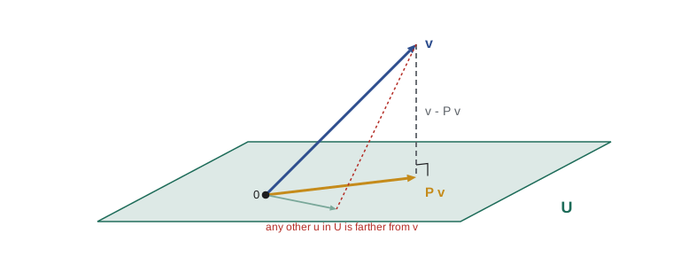
Lesson 9 showed that every vector splits uniquely into a piece in a subspace \(U\) and a piece orthogonal to it. The first piece is the orthogonal projection of the vector onto \(U\), and it is the closest point of \(U\) to the vector. That single fact drives an enormous range of applications: fitting lines and curves to data, approximating functions by polynomials or trigonometric sums, compressing signals, and solving inconsistent linear systems. MATH-125 met least squares through the normal equations. This lesson treats projections as operators, proves the best approximation theorem in any inner product space, and shows why the QR factorization, rather than the normal equations, is how least squares problems are solved in practice.
Projection operators
Let \(U\) be a finite-dimensional subspace of an inner product space \(V\). The orthogonal projection onto \(U\) is the map \(P_U : V \to V\) that sends \(\mathbf{v}\) to its component in \(U\) in the decomposition \(V = U \oplus U^{\perp}\). If \(\mathbf{e}_1, \dots, \mathbf{e}_m\) is an orthonormal basis of \(U\), then
the matrix form holding in \(\mathbb{R}^n\) with the dot product. Its basic properties follow straight from the definition: \(P_U\) is linear; its image is \(U\) and its kernel is \(U^{\perp}\); it fixes \(U\) pointwise, so \(P_U^2 = P_U\); it is self-adjoint; \(I - P_U = P_{U^{\perp}}\); and \(\|P_U\mathbf{v}\| \le \|\mathbf{v}\|\), by Pythagoras.
Theorem. An operator \(P\) on a finite-dimensional inner product space is an orthogonal projection (onto its image) exactly when \(P^2 = P\) and \(P^{*} = P\). Proof: we have seen the forward direction. Conversely, if \(P^2 = P\) then every \(\mathbf{v}\) is \(P\mathbf{v} + (\mathbf{v} - P\mathbf{v})\) with the first piece in \(\operatorname{im}P\) and the second in \(\ker P\). If also \(P^{*} = P\), then \(\ker P = \ker P^{*} = (\operatorname{im}P)^{\perp}\), so the decomposition is the orthogonal one. Without self-adjointness, \(P^2 = P\) gives an oblique projection, along a complement that need not be perpendicular, like the shadow cast by a low sun.
In the language of lesson 7, \(P^2 = P\) means the minimal polynomial divides \(x(x - 1)\), so a projection is diagonalizable with eigenvalues 0 and 1. Its trace is therefore its rank, the dimension of \(U\), a fact used constantly in statistics, where the trace of the hat matrix counts the parameters of a regression model.
The best approximation theorem
Theorem. For every \(\mathbf{v} \in V\) and every \(\mathbf{u} \in U\), \(\|\mathbf{v} - P_U\mathbf{v}\| \le \|\mathbf{v} - \mathbf{u}\|\), with equality only when \(\mathbf{u} = P_U\mathbf{v}\).
Proof. Write \(\mathbf{v} - \mathbf{u} = (\mathbf{v} - P_U\mathbf{v}) + (P_U\mathbf{v} - \mathbf{u})\). The first piece is in \(U^{\perp}\) and the second is in \(U\), so they are orthogonal and Pythagoras gives \(\|\mathbf{v} - \mathbf{u}\|^2 = \|\mathbf{v} - P_U\mathbf{v}\|^2 + \|P_U\mathbf{v} - \mathbf{u}\|^2\). The second term is positive unless \(\mathbf{u} = P_U\mathbf{v}\).
The theorem says nothing about \(\mathbb{R}^n\); it works in any inner product space. In \(C[-\pi, \pi]\) with \(\langle f, g \rangle = \int fg\), the functions \(1, \cos t, \sin t, \dots, \cos nt, \sin nt\) are orthogonal, and projecting onto their span gives the trigonometric polynomial of degree \(n\) closest to \(f\) in the mean-square sense. Its coefficients are the Fourier coefficients \(\langle f, \cos kt \rangle/\langle \cos kt, \cos kt \rangle\) and so on. Bessel's inequality, \(\|P_U f\| \le \|f\|\), says the sum of the squared Fourier coefficients (suitably weighted) is at most \(\int f^2\). In \(P_n\) with the integral inner product on \([-1, 1]\), the Legendre polynomials of lesson 9 play the same role.
Worked problem
The best linear approximation to a function
Find the polynomial \(p(t) = a + bt\) minimizing \(\int_{-1}^{1}(e^t - p(t))^2\,dt\).
Show solution
- The orthogonal basis \(1, t\) of \(P_1\) has \(\langle 1, 1 \rangle = 2\) and \(\langle t, t \rangle = 2/3\).
- \(\langle e^t, 1 \rangle = \int_{-1}^{1}e^t\,dt = e - e^{-1}\).
- \(\langle e^t, t \rangle = \int_{-1}^{1}te^t\,dt = \big[(t - 1)e^t\big]_{-1}^{1} = 2e^{-1}\).
- So \(a = (e - e^{-1})/2 = \sinh 1 \approx 1.1752\) and \(b = 2e^{-1}/(2/3) = 3e^{-1} \approx 1.1036\).
Answer: \(p(t) \approx 1.1752 + 1.1036t\). Unlike the Taylor polynomial \(1 + t\), which is excellent near 0 and poor at the ends, this line spreads the error evenly over the whole interval.
Least squares
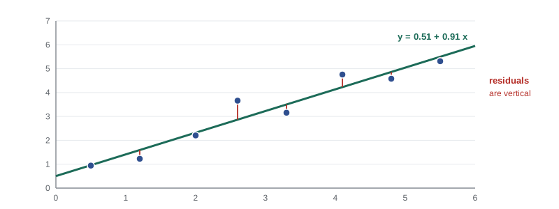
Now let \(A\) be an \(m \times n\) real matrix with \(m > n\) and let \(\mathbf{b} \in \mathbb{R}^m\). The system \(A\mathbf{x} = \mathbf{b}\) usually has no solution, so we seek \(\hat{\mathbf{x}}\) minimizing \(\|A\mathbf{x} - \mathbf{b}\|\). Since \(A\mathbf{x}\) ranges over the column space \(U = \operatorname{im}A\), the best approximation theorem says \(A\hat{\mathbf{x}} = P_U\mathbf{b}\), and the residual \(\mathbf{b} - A\hat{\mathbf{x}}\) lies in \(U^{\perp} = \ker A^{T}\). That gives the normal equations
which have a unique solution exactly when the columns of \(A\) are independent, because \(\ker A^{T}A = \ker A\) (if \(A^{T}A\mathbf{x} = \mathbf{0}\) then \(\|A\mathbf{x}\|^2 = \mathbf{x}^{T}A^{T}A\mathbf{x} = 0\)). In that case \(P_U = A(A^{T}A)^{-1}A^{T}\), the hat matrix of regression. The least squares line, the polynomial fits and the multiple regression models of AI-210 are all this one formula with different matrices \(A\).
The QR factorization
Apply Gram–Schmidt to the columns \(\mathbf{a}_1, \dots, \mathbf{a}_n\) of \(A\), assumed independent. Each \(\mathbf{a}_k\) is a combination of \(\mathbf{q}_1, \dots, \mathbf{q}_k\), with coefficients \(r_{jk} = \langle \mathbf{a}_k, \mathbf{q}_j \rangle\) for \(j < k\) and \(r_{kk} = \|\mathbf{w}_k\| > 0\). Collecting these,
This is the reduced QR factorization; it is unique under the positivity condition. For least squares it is ideal. Substituting into the normal equations, \(R^{T}Q^{T}QR\hat{\mathbf{x}} = R^{T}Q^{T}\mathbf{b}\), and since \(R^{T}\) is invertible this simplifies to
a triangular system solved by back substitution. The matrix \(A^{T}A\) is never formed. That matters because of conditioning. The condition number \(\kappa(A) = \sigma_{\max}/\sigma_{\min}\), defined through singular values in lesson 12, measures how much relative errors in the data can be amplified. Forming \(A^{T}A\) squares it: \(\kappa(A^{T}A) = \kappa(A)^2\). If \(\kappa(A) = 10^8\), the normal equations have condition number \(10^{16}\) and in double precision the answer can lose every digit; QR works with \(\kappa(A)\) itself.
Householder reflections
Production software computes QR not by Gram–Schmidt but by Householder reflections. For a unit vector \(\mathbf{u}\), the matrix \(H = I - 2\mathbf{u}\mathbf{u}^{T}\) reflects \(\mathbb{R}^m\) across the hyperplane \(\mathbf{u}^{\perp}\); it is symmetric, orthogonal and its own inverse. Given a vector \(\mathbf{x}\), choosing \(\mathbf{u}\) parallel to \(\mathbf{x} \pm \|\mathbf{x}\|\mathbf{e}_1\) gives \(H\mathbf{x} = \mp\|\mathbf{x}\|\mathbf{e}_1\), zeroing every entry below the first. Applying such reflections column by column reduces \(A\) to triangular form: \(H_n\cdots H_1A = R\), so \(A = QR\) with \(Q = H_1\cdots H_n\) exactly orthogonal up to rounding. Because each step is an orthogonal transformation, which preserves lengths, errors are not amplified. This is the algorithm behind numpy's qr and behind the QR iteration for eigenvalues sketched in lesson 5.
| Method | Work for m by n | Error depends on | When to use |
|---|---|---|---|
| Normal equations with Cholesky | about \(mn^2 + n^3/3\) | \(\kappa(A)^2\) | Well-conditioned problems where speed matters |
| Classical Gram–Schmidt QR | about \(2mn^2\) | Unstable for nearly dependent columns | Rarely; mainly for teaching |
| Householder QR | about \(2mn^2 - 2n^3/3\) | \(\kappa(A)\) and the residual size | The default for dense least squares |
| SVD (lesson 12) | Several times QR | \(\kappa(A)\); handles rank deficiency | Rank-deficient or very ill-conditioned problems |
Normal equations versus QR in practice
The code fits polynomials of increasing degree to noisy samples of a smooth function, using a Vandermonde matrix whose condition number grows quickly with the degree. It solves each problem with the normal equations and with QR and compares both with numpy's SVD-based lstsq as a reference.
import numpy as np
rng = np.random.default_rng(221)

t = np.linspace(0, 1, 40)
y = np.cos(3 * t) + 0.001 * rng.standard_normal(t.size)

for deg in (3, 8, 13):
    A = np.vander(t, deg + 1, increasing=True)
    ref = np.linalg.lstsq(A, y, rcond=None)[0]
    x_ne = np.linalg.solve(A.T @ A, A.T @ y)
    Q, R = np.linalg.qr(A)
    x_qr = np.linalg.solve(R, Q.T @ y)        # R is triangular; solve() is fine for a demo
    err = lambda x: np.linalg.norm(x - ref) / np.linalg.norm(ref)
    print(f"degree {deg:2d}: cond(A) = {np.linalg.cond(A):.1e}, cond(A^T A) = {np.linalg.cond(A.T @ A):.1e}")
    print(f"           relative error: normal equations {err(x_ne):.1e}, QR {err(x_qr):.1e}")

# the projection matrix is idempotent and symmetric, with trace equal to the rank
A = np.vander(t, 4, increasing=True)
Q, _ = np.linalg.qr(A)
P = Q @ Q.T
print("P^2 = P:", np.allclose(P @ P, P), " P^T = P:", np.allclose(P.T, P), " trace(P) =", round(np.trace(P), 10))
r = y - P @ y
print("residual orthogonal to the columns:", np.allclose(A.T @ r, 0, atol=1e-12))degree 3: cond(A) = 1.2e+02, cond(A^T A) = 1.4e+04
relative error: normal equations 7.0e-14, QR 3.2e-16
degree 8: cond(A) = 6.2e+05, cond(A^T A) = 3.8e+11
relative error: normal equations 6.0e-06, QR 4.8e-14
degree 13: cond(A) = 4.1e+09, cond(A^T A) = 2.4e+17
relative error: normal equations 9.7e-01, QR 2.1e-13
P^2 = P: True P^T = P: True trace(P) = 4.0
residual orthogonal to the columns: TrueFor degree 3 both methods agree to many digits. By degree 13 the Gram matrix \(A^{T}A\) has a condition number near or beyond the reciprocal of machine precision, and the normal-equation coefficients have lost most of their accuracy, while QR remains close to the reference. The final lines confirm the operator facts: the projection matrix is idempotent and symmetric, its trace is the number of fitted parameters, and the residual is orthogonal to every column.
The geometry also explains the familiar coefficient of determination. If the model includes a constant column, center the data so that \(\bar y = 0\). Then \(\mathbf{b} = P\mathbf{b} + (\mathbf{b} - P\mathbf{b})\) is an orthogonal decomposition, Pythagoras gives \(\|\mathbf{b}\|^2 = \|P\mathbf{b}\|^2 + \|\mathbf{b} - P\mathbf{b}\|^2\), and \(R^2 = \|P\mathbf{b}\|^2/\|\mathbf{b}\|^2\) is the squared cosine of the angle between the data vector and the column space. Adding a column can only enlarge the column space and so can only shrink the angle, which is why \(R^2\) never decreases when a predictor is added, however useless that predictor is. Statisticians correct for this with adjusted \(R^2\), whose penalty is the trace of the projection, the number of parameters.
Weighted and constrained variants
If some observations are more reliable than others, minimize \(\sum w_i(b_i - (A\mathbf{x})_i)^2\) instead. That is ordinary least squares in the weighted inner product \(\langle \mathbf{u}, \mathbf{v} \rangle_W = \mathbf{u}^{T}W\mathbf{v}\), and the normal equations become \(A^{T}WA\hat{\mathbf{x}} = A^{T}W\mathbf{b}\). Rescaling rows by \(\sqrt{w_i}\) turns it back into an ordinary problem, which can then be solved by QR. Adding a penalty \(\lambda\|\mathbf{x}\|^2\) gives ridge regression, \((A^{T}A + \lambda I)\hat{\mathbf{x}} = A^{T}\mathbf{b}\), which is always solvable for \(\lambda > 0\) and which lesson 12 interprets through singular values. In computer graphics (CMPUT-411), least squares fits are used to register point clouds and to smooth meshes; in robotics and vision (CMPUT-367) they estimate camera parameters from point correspondences.
Common mistakes
MistakeThinking every matrix with \(P^2 = P\) is an orthogonal projection.
InsteadIt must also be self-adjoint; otherwise it is an oblique projection.
MistakeUsing \(P = AA^{T}\) when the columns of \(A\) are not orthonormal.
InsteadUse \(A(A^{T}A)^{-1}A^{T}\), or \(QQ^{T}\) with \(Q\) from a QR factorization.
MistakeSolving least squares by forming \(A^{T}A\) for an ill-conditioned \(A\).
InsteadUse QR or the SVD; the normal equations square the condition number.
MistakeMinimizing the perpendicular distances to a line when fitting \(y\) on \(x\).
InsteadOrdinary least squares minimizes vertical residuals; perpendicular distances lead to total least squares, solved by the SVD.
MistakeForgetting that the residual is orthogonal to the column space.
Instead\(A^{T}(\mathbf{b} - A\hat{\mathbf{x}}) = \mathbf{0}\) is the defining condition.
Summary and key terms
- The orthogonal projection onto \(U\) is \(\sum\langle \mathbf{v}, \mathbf{e}_j \rangle\mathbf{e}_j\), or \(QQ^{T}\) in matrix form.
- Orthogonal projections are exactly the operators with \(P^2 = P = P^{*}\); their trace is their rank.
- The projection is the unique closest point of \(U\), in any inner product space.
- Fourier and Legendre approximations are projections in function spaces.
- Least squares solutions satisfy \(A^{T}A\hat{\mathbf{x}} = A^{T}\mathbf{b}\), or \(R\hat{\mathbf{x}} = Q^{T}\mathbf{b}\) with \(A = QR\).
- QR avoids squaring the condition number and is the standard method; Householder reflections compute it stably.
- orthogonal projection
- The map sending \(\mathbf{v}\) to its component in \(U\) along \(U^{\perp}\).
- idempotent
- Satisfying \(P^2 = P\).
- best approximation theorem
- The projection is the unique closest point of the subspace.
- normal equations
- \(A^{T}A\hat{\mathbf{x}} = A^{T}\mathbf{b}\).
- QR factorization
- \(A = QR\) with orthonormal columns in \(Q\) and upper triangular \(R\).
- Householder reflection
- \(I - 2\mathbf{u}\mathbf{u}^{T}\) for a unit vector \(\mathbf{u}\).
- condition number
- A measure of how much relative errors in data can be amplified.
- hat matrix
- The projection \(A(A^{T}A)^{-1}A^{T}\) onto the column space.
Practice problems
Work each problem on paper first, then reveal the answer to check.
Find the projection matrix onto the line spanned by \((1, 2, 2)\).
Show answer
\(\frac19\begin{pmatrix} 1 & 2 & 2 \\ 2 & 4 & 4 \\ 2 & 4 & 4 \end{pmatrix}\).
Prove that if \(P\) is an orthogonal projection then so is \(I - P\).
Show answer
\((I - P)^2 = I - 2P + P^2 = I - P\) and \((I - P)^{*} = I - P\).
Prove that \(\|P\mathbf{v}\| \le \|\mathbf{v}\|\) for an orthogonal projection.
Show answer
\(\|\mathbf{v}\|^2 = \|P\mathbf{v}\|^2 + \|\mathbf{v} - P\mathbf{v}\|^2\) by Pythagoras.
Fit \(y = a + bx\) to \((0, 1), (1, 3), (2, 4)\).
Show answer
Normal equations \(3a + 3b = 8\), \(3a + 5b = 11\); \(b = 1.5\), \(a = 7/6\).
Show that a Householder matrix is orthogonal and symmetric.
Show answer
\(H^{T} = H\) clearly, and \(H^2 = I - 4\mathbf{u}\mathbf{u}^{T} + 4\mathbf{u}(\mathbf{u}^{T}\mathbf{u})\mathbf{u}^{T} = I\).
Prove that \(\ker A^{T}A = \ker A\).
Show answer
If \(A^{T}A\mathbf{x} = 0\) then \(\|A\mathbf{x}\|^2 = \mathbf{x}^{T}A^{T}A\mathbf{x} = 0\); the other inclusion is clear.
Lesson quiz · 5 questions
Score 60% or more to complete this lesson.
Create a free account to save your progress, take quizzes and earn a certificate.