Side-scan sonar

The shore of Commencement Bay has been industrial for more than a century. Old wharves and mills were built, extended, burned and replaced; piles were cut off at the mud line or simply abandoned; cables, anchors and the odd sunken barge lie where they fell. Multibeam measures the shape of the seabed well, but small, low objects can hide among its soundings, especially in the outer beams. So Mira's plan adds side-scan sonar over the whole berth pocket: an acoustic image of the seabed in which objects stand out by their echoes and, even more, by the shadows they cast.

How side-scan sonar works

A side-scan sonar has a transducer on each side of a streamlined towfish or of a hull mount. Each transducer sends a fan-shaped pulse, very narrow along track (a fraction of a degree) and wide in the vertical plane, sideways and down toward the seabed. As the pulse sweeps outward across the bottom, the transducer records the strength of the returning echo against time. Rough or hard patches, and the sides of objects facing the sonar, return strong echoes; smooth mud returns weak ones; and areas hidden behind objects, which the sound cannot reach, return nothing at all, leaving acoustic shadows. Each ping becomes one line of an image; as the towfish moves forward, the lines build up a picture of a strip of seabed on each side of the track.

Side-scan sonars operate at frequencies from about 100 kHz, for wide coverage, to 1 MHz or more, for very fine detail at short range. Many systems transmit two frequencies at once, one for reconnaissance and one for identification. The along-track resolution is set by the horizontal beam width multiplied by the range, so it degrades away from the towfish; the across-track resolution is set by the pulse length or bandwidth and is much finer. Synthetic aperture sonar, which combines many pings coherently as the towfish moves, keeps a fine along-track resolution to long range and is now used for demanding searches.

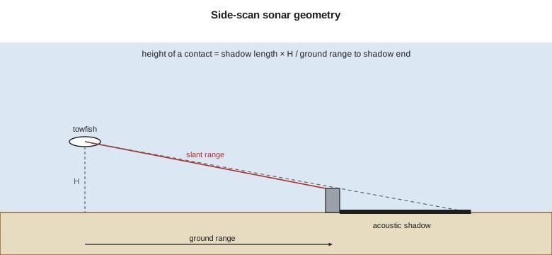
Geometry: slant range, ground range and height

The sonar measures slant range, the straight-line distance from the transducer to each point on the seabed. Near the towfish, the slant range differs greatly from the horizontal or ground range; far away, they converge. Converting slant range to ground range assumes a flat seabed at the towfish's height \(H\) above it:

The first echo from the seabed arrives at a slant range equal to \(H\), so the record directly beneath the towfish is a blank water column, the nadir gap, which must be covered by adjacent lines or by the multibeam. An object of height \(h\) casts a shadow behind it. By similar triangles, if the ground range from the towfish to the end of the shadow is \(R\) and the shadow's length is \(L_s\),

so the shadow's length gives the object's height, provided the towfish height is known and the seabed is roughly flat. Height estimates from side-scan are approximate, good to perhaps tens of percent, and they are no substitute for a least depth from multibeam, but they rank contacts quickly: a contact with a long shadow far from the towfish is worth developing.

import math
# Towfish 6.0 m above the seabed; slant ranges to a contact and to the end of its acoustic shadow
H = 6.0
slant_target, slant_shadow_end = 31.0, 36.4
gr_t = math.sqrt(slant_target ** 2 - H ** 2)        # slant-range correction to ground range
gr_s = math.sqrt(slant_shadow_end ** 2 - H ** 2)
Ls = gr_s - gr_t
h = Ls * H / gr_s                                     # similar triangles: height from shadow length
print(f"ground range to the contact {gr_t:.2f} m, shadow length {Ls:.2f} m, height about {h:.2f} m")
print(f"slant range overstates ground range by {slant_target - gr_t:.2f} m here")

# Layback: towfish position from the vessel's antenna by cable out and depth
cable, fish_depth, antenna_to_tow = 42.0, 11.0, 7.5
lay = math.sqrt(cable ** 2 - fish_depth ** 2) + antenna_to_tow
print(f"layback about {lay:.1f} m behind the antenna (cable catenary ignored)")

# How many pings hit a 1 m object at the outer range, given speed and range scale?
c = 1485.0
for rng, kn in ((50, 4.0), (50, 6.0), (100, 4.0)):
    rate = c / (2 * rng)                               # one ping per round trip to the range limit
    v = kn * 0.5144
    hits = 1.0 / (v / rate)
    beam_along = math.radians(0.3) * rng               # along-track beam width at the far range
    print(f"range {rng:3d} m at {kn:.0f} kn: {rate:4.1f} pings/s, {v/rate:.2f} m between pings, "
          f"{hits:4.1f} pings on 1 m; beam {beam_along:.2f} m wide along track at the far edge")

# Line spacing for 200 % coverage with a 50 m range scale and a 10 m nadir gap filled by the other lines
rng, gap = 50.0, 2 * H
print(f"200 % side-scan coverage: line spacing about {rng - gap/2:.0f} m (each point seen from two lines)")

ground range to the contact 30.41 m, shadow length 5.49 m, height about 0.92 m
slant range overstates ground range by 0.59 m here
layback about 48.0 m behind the antenna (cable catenary ignored)
range  50 m at 4 kn: 14.8 pings/s, 0.14 m between pings,  7.2 pings on 1 m; beam 0.26 m wide along track at the far edge
range  50 m at 6 kn: 14.8 pings/s, 0.21 m between pings,  4.8 pings on 1 m; beam 0.26 m wide along track at the far edge
range 100 m at 4 kn:  7.4 pings/s, 0.28 m between pings,  3.6 pings on 1 m; beam 0.52 m wide along track at the far edge
200 % side-scan coverage: line spacing about 44 m (each point seen from two lines)

A contact at 31.0 m slant range with its shadow ending at 36.4 m, from a towfish 6.0 m above the seabed, lies 30.4 m out in ground range and stands about 0.9 m high: perhaps a pile stub, perhaps a block of debris. At a 50 m range scale the sonar can ping about 15 times a second; at 4 knots that puts about seven pings on a one-meter object, enough to see it clearly, but at 6 knots only about five, and at 100 m range only about four. That is why side-scan surveys searching for small objects use short ranges and modest speeds, and why charting specifications state minimum numbers of pings on a target of a given size.

Towing and positioning

A towed sonar is decoupled from the vessel's motion and can be flown close to the seabed, which lengthens shadows and improves the image, but its position is not known directly. The simplest estimate is layback: the towfish lies behind the tow point by roughly the horizontal component of the cable length, calculated from the cable paid out and the towfish's depth from its pressure sensor. On the berth, with 42 m of cable and the towfish 11 m deep, the layback is about 48 m behind the antenna. Currents push the towfish off to one side and the cable sags in a curve, so layback alone can be off by meters; for precise work, an acoustic positioning system tracks the towfish from the vessel. Hull-mounted and pole-mounted side-scans avoid the problem at the cost of flying higher above the seabed, and many modern multibeams produce a side-scan-like image from their own backscatter.

The towfish's height above the seabed is usually set at about 10 percent of the range scale, a compromise between shadow length and the risk of hitting the bottom or an obstruction. In a harbor, with cables, piles and moored ships, a towed system is a hazard in itself, and Grant flies the towfish higher near the wharf face and switches to the hull-mounted side-scan on the launch's pole for the last few lines.

Coverage and line planning

Side-scan coverage is planned in percent like multibeam coverage. With a 50 m range scale on each side, a line covers about 100 m of seabed minus the nadir gap. For 200 percent coverage, lines are spaced so that every point of the seabed is imaged from two lines, ideally from opposite directions so that an object's shadow falls on different sides; that also fills each line's nadir gap with the outer range of the neighboring lines. The berth survey uses a 50 m range scale and lines about 40 to 45 m apart, run on the same days as the multibeam where possible.

Side-scan and multibeam together

Side-scan and multibeam answer different questions. Multibeam measures depth and shape with known uncertainty; side-scan detects and images objects with great sensitivity but measures depth poorly. Charting specifications have long allowed object detection to be met either by high-density multibeam or by side-scan coverage with multibeam development of the contacts, and many surveys use both. The combination is strongest when the two are interpreted together: a side-scan contact with no matching multibeam anomaly may be a soft feature, such as a patch of kelp or a tire lying flat, or it may be an object the multibeam's footprint averaged away; a multibeam spike with no side-scan contact may be noise. Leah overlays the side-scan mosaic, the backscatter mosaic and the multibeam surface in the processing software, so that every contact can be judged against all three, and records the outcome of each comparison in the contact list delivered with the survey.

Interpreting the record

Reading a side-scan record is a skill learned by experience. The interpreter scans the waterfall display, the scrolling image, and the mosaic built from all the lines, looking for contacts: anything that stands up from the seabed, casts a shadow, returns an unusually strong echo or breaks a pattern. Each contact is measured (position, length, width, shadow height), described, classified and cross-checked against the multibeam surface and the backscatter mosaic. Some patterns are familiar: sand waves and ripples, trawl marks and anchor scars, cables as thin straight lines, piles as bright dots with short shadows, wrecks as complex shapes with long shadows, fish schools as clouds in the water column. Others need a second look from another direction or a closer, higher-frequency pass.

On the berth, Theo and Mira log 61 contacts. Most are debris and cut piles; eleven stand more than half a meter above the seabed and are flagged for multibeam development; one, a long, straight, slightly curved feature 0.3 m high, runs diagonally across the pocket. It does not appear on any of the terminal's drawings. A search of old records turns up a decommissioned water line from a long-gone cannery, and the client arranges for it to be located by divers and removed before dredging.

Side-scan in fresh water

Side-scan sonar is also widely used inland: to inspect dams, intakes and bridge piers, to find debris before dredging, to map habitat, and in search and recovery. For the Sun River intake, Grant runs a small hull-mounted side-scan along the reach to check for boulders and debris near the proposed intake screen; in the shallow, clear water it gives a sharp image of the cobble bed and of an old car body that the project's crew remove before construction.