Multibeam sonar

Northshore's survey launch is a ten-meter aluminum catamaran with a multibeam echo sounder mounted on a rigid pole between the hulls. Its transducers form 512 beams across a fan of up to 130°, each about 1° wide, and ping up to fifty times a second. In a morning on the berth it collects more depth measurements than a single-beam crew could gather in a year. Ines has processed lidar point clouds for years, and the multibeam's output looks familiar to her: a dense cloud of points with intensities. What is new is the physics behind each point, and the way the geometry of a swath determines what the survey can and cannot see.

Beam forming

A multibeam echo sounder uses two arrays of transducer elements, usually arranged in a cross (a Mills cross): a transmit array along the vessel's keel that sends a pulse narrow in the along-track direction and wide across track, and a receive array across the keel that listens in many narrow directions at once. By adding the signals from the receive elements with carefully chosen delays or phase shifts, the processor forms beams pointing at different angles across the fan, a technique called beam forming. Each beam is narrow across track because of the receive array and narrow along track because of the transmit array; their intersection is a small patch of seabed for each beam.

For each beam, the system detects when the echo arrives. Near nadir, where the echo is strong and short, it uses the time of peak amplitude; toward the outer beams, where the echo is long and smeared across the footprint, it uses phase detection, comparing the phase of the signal on two halves of the receive array to find the precise instant when the echo comes from the beam's center direction. The output for each ping is a list of beam angles and two-way travel times, which the system converts to depths and across-track distances by ray tracing through the sound speed profile (Lesson 3).

Swath width and coverage

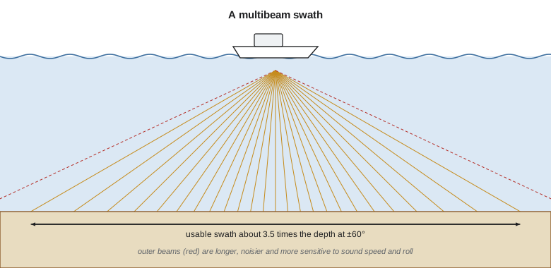
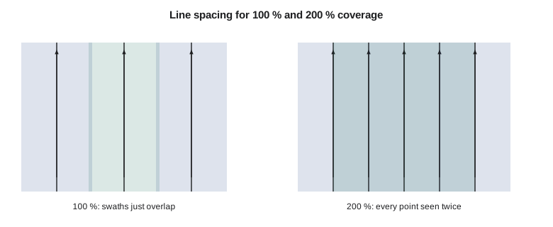
The width of seabed covered by one ping, the swath, grows with depth and with the angular sector: for a flat bottom, \(W = 2d\tan(\theta/2)\). A 130° sector covers about 4.3 times the depth; but outer beams are long, weak and sensitive to sound speed and roll, so for high-order work surveyors usually keep only the beams within about ±60°, a swath of about 3.5 times the depth. The line spacing follows from the usable swath and the required coverage. For 100 percent coverage, adjacent swaths overlap a little, often 10 to 20 percent, to allow for steering errors and to give overlap for checking; for 200 percent coverage, every point of the seabed is seen from two lines, which doubles the effort but gives redundancy for detecting objects and errors.

Shallow water is expensive to survey with multibeam because the swath shrinks with depth. In 17 m the usable swath is about 59 m; in 3 m it is under 11 m, and lines must be run five or six times closer together. That is why the shallow margins of a harbor or a reservoir take a disproportionate share of a survey's time, and why topobathymetric lidar or an uncrewed vessel (Lesson 12) is attractive there.

Ping rate and sounding density

A multibeam cannot ping again until the echoes from the previous ping have returned from the outermost beams, so the maximum ping rate falls as depth increases. In 8 m of water the launch's system can ping about 33 times a second; in 25 m, about 12. Modern systems also transmit several pings in the water at once, or split the swath into sectors with different frequencies, to raise the rate. The along-track spacing of soundings is the vessel speed divided by the ping rate, and the across-track spacing depends on the number of beams, their arrangement (equiangular or equidistant) and the beam angle. Together they give the sounding density, which, with the footprint size, decides whether small objects can be detected.

import math
# Multibeam on the harbour launch: 512 beams over a 130 degree sector, 1 x 1 degree beams
sector, nbeams, bw = 130.0, 512, 1.0
c = 1485.0
for depth in (8.0, 17.0, 25.0):
    swath = 2 * depth * math.tan(math.radians(sector / 2))
    # Ping rate is limited by the two-way travel time to the outermost beam
    slant = depth / math.cos(math.radians(sector / 2))
    rate = min(50.0, 1.0 / (2 * slant / c + 0.005))
    print(f"depth {depth:4.1f} m: swath {swath:6.1f} m ({swath/depth:.1f} x depth), max ping rate {rate:4.1f} Hz")

# Line spacing for 100 % and 200 % coverage in 17 m, keeping only beams within +/-60 degrees
depth, usable = 17.0, 60.0
w = 2 * depth * math.tan(math.radians(usable))
print(f"usable swath {w:.1f} m; spacing {0.9*w:.1f} m for 100 % with 10 % overlap, {w/2:.1f} m for 200 %")

# Along-track and across-track sounding spacing, and soundings on a 1 m cube
speed = 6.0 * 0.5144        # 6 knots in m/s
slant = depth / math.cos(math.radians(sector / 2))
rate = min(50.0, 1.0 / (2 * slant / c + 0.005))
along = speed / rate
print(f"at 6 kn and {rate:.1f} Hz: {along:.2f} m between pings")
for ang in (0.0, 30.0, 60.0):
    a = math.radians(ang)
    fp_across = depth * math.radians(bw) / math.cos(a) ** 2
    spacing = depth * (math.radians(sector) / nbeams) / math.cos(a) ** 2   # equiangular beams on a flat bottom
    fp_along = depth * math.radians(bw) / math.cos(a)
    hits = max(1, int(1.0 / along)) * max(1, int(1.0 / spacing))
    print(f"beam at {ang:4.1f} deg: footprint {fp_across:.2f} m across x {fp_along:.2f} m along, "
          f"beam spacing {spacing:.2f} m, about {hits} soundings on a 1 m cube")

# Area coverage rate for a day of survey
lines_km = 6 * 3600 * speed / 1000 * 0.85     # 6 h on line, 85 % efficiency
print(f"one day: {lines_km:.0f} km of line, about {lines_km * 0.9 * w / 1000:.2f} km2 at 100 % coverage in 17 m")

depth  8.0 m: swath   34.3 m (4.3 x depth), max ping rate 32.8 Hz
depth 17.0 m: swath   72.9 m (4.3 x depth), max ping rate 16.9 Hz
depth 25.0 m: swath  107.2 m (4.3 x depth), max ping rate 11.8 Hz
usable swath 58.9 m; spacing 53.0 m for 100 % with 10 % overlap, 29.4 m for 200 %
at 6 kn and 16.9 Hz: 0.18 m between pings
beam at  0.0 deg: footprint 0.30 m across x 0.30 m along, beam spacing 0.08 m, about 65 soundings on a 1 m cube
beam at 30.0 deg: footprint 0.40 m across x 0.34 m along, beam spacing 0.10 m, about 45 soundings on a 1 m cube
beam at 60.0 deg: footprint 1.19 m across x 0.59 m along, beam spacing 0.30 m, about 15 soundings on a 1 m cube
one day: 57 km of line, about 3.00 km2 at 100 % coverage in 17 m

At 17 m depth and 6 knots, the launch pings about 17 times a second, 0.18 m apart along track. Near nadir the beam footprint is 0.30 m square and the beams fall 0.08 m apart across track, putting about 65 soundings on a 1 m cube; at 60° the footprint has stretched to 1.19 m across track and 0.59 m along, and only about 15 soundings land on the cube. A day of six hours on line at 85 percent efficiency gives about 57 km of line and 3.0 km² at 100 percent coverage in this depth: the berth pocket and its approach, about 0.6 km² together, can be covered at 200 percent in well under a day, leaving time for cross lines, calibration and the shallow margins.

Detecting objects

Charting authorities require that significant objects be detected, not just that the bottom be measured. IHO S-44 states feature detection in terms of cubes: in its higher orders, a survey must be able to detect cubic features of 1 m or 0.5 m on a side (Lesson 10). National specifications translate this into rules for sounding density and footprint size, for instance by requiring a minimum number of soundings on such a cube, so that the object rises out of the surrounding seabed in the data. Objects detected in the data are then developed: the launch runs extra lines over them, at slower speed and with the object near nadir, to find the least depth over them.

Detection depends on more than density. The outer beams' large footprints average a small object with the seabed around it; a mast or a pile standing up from the bottom may return only a few soundings before the beams pass it; and acoustic shadows behind objects hide what lies beyond. Side-scan sonar (Lesson 9) complements multibeam for this reason. Mira's plan for the berth calls for 200 percent multibeam coverage with nadir-to-60° beams, and side-scan sonar over the pocket, because the old harbor may contain debris from the wharves that once stood there.

Backscatter and water column

Besides depth, each beam records the strength of the echo, its backscatter. Backscatter depends on the seabed's roughness and hardness and on the angle at which the sound strikes it: rock and gravel return strongly, soft mud weakly. Mosaicked across a survey, corrected for angle and range, backscatter becomes an image of the seabed that helps classify it into sediment types, which is valuable for dredging (hard material is expensive to remove) and for habitat mapping. Many multibeams also record the water column, the echoes from the entire fan between the transducer and the seabed, revealing fish, gas plumes, kelp and the masts of wrecks.

Installation and integration

A multibeam is only as good as its integration with the systems around it. The transducer must be rigidly mounted, its position relative to the GNSS antennas and the motion sensor measured precisely in the vessel's reference frame, and its alignment angles determined by calibration (Lesson 7). All sensors must share one time base, usually GNSS time distributed with a pulse-per-second signal, because a millisecond of timing error at a roll rate of a few degrees per second produces a measurable error in the outer beams. Surface sound speed must reach the beam former continuously. Before the survey, Mira and Grant spend a day on the dimensional survey of the launch with a total station, measuring every offset to the nearest centimeter, and another day on calibration.

Real-time quality control

During acquisition, the hydrographer watches several displays: the swath profile, which should be flat across a flat seabed; a coverage map building up behind the vessel; the motion and position quality indicators; and the difference between the surface sound speed sensor and the profile. Many systems display a real-time surface gridded from the incoming data, colored by depth or by the standard deviation of soundings in each cell, which lets the operator see gaps, artifacts and noisy areas while the launch is still there to fix them. Lines with problems are rerun the same day; finding a gap in the office a week later costs a mobilization.

Choosing a system

Multibeams are built for depth ranges. Shallow-water systems at 200 to 700 kHz work from about half a meter to a few hundred meters; mid-water systems at tens of kilohertz reach a few thousand meters; and deep-water systems at 12 kHz map the ocean floor from large ships. Within a class, systems differ in beam count, beam width, maximum sector, ping rate, whether they can steer the swath to compensate for pitch and yaw, and how they handle multiple pings in the water. For the berth, a shallow-water system with 1° beams is ideal; for the reservoir margins, a compact system on an uncrewed vessel; for the river, where depths are under three meters, single-beam sections and RTK are more practical.