Grid and ground distances

The question that started this course, why the GIS length of Lateral 7 was 0.7 m per kilometer shorter than the length taped in the field, is answered in this lesson. Two effects combine. The state plane projection's scale factor shrinks lengths on the grid by about 570 ppm at the district, and the height of the ground above the ellipsoid makes every ground distance about 160 ppm longer than the same distance on the ellipsoid. Together they make grid distances about 730 ppm shorter than ground distances. Surveyors handle this with the combined scale factor, and engineers who want grid and ground to agree use a low-distortion projection. Both are explained here.

Three surfaces and three distances

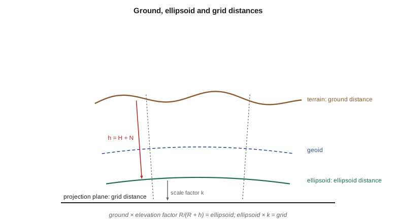
A distance measured with a total station is a slope distance between the instrument and the prism. The instrument's software reduces it to a horizontal distance using the measured zenith angle, and that horizontal distance lies, roughly, at the mean height of the two ends: it is a ground distance. Geodetic computations use the length of the same line on the ellipsoid, the ellipsoid distance, which is shorter because the ellipsoid lies beneath the ground and the lines from the two ends to the Earth's center converge. Projected coordinates give a third length, the grid distance, which differs from the ellipsoid distance by the projection's scale factor. Converting between ground and grid requires both steps.

The elevation factor

Over short lines the ground and the ellipsoid can be treated as concentric spheres of radii \(R + h\) and \(R\), so that

where \(h\) is the mean ellipsoidal height of the line and \(R\) a radius of curvature for the line's location and direction. The Gaussian mean radius \(\sqrt{MN}\) is the usual choice; using the radius in the line's direction changes the factor by less than 0.1 ppm for lines of a few kilometers. The height must be the ellipsoidal height, \(h = H + N\), not the orthometric height \(H\) read from a map or a benchmark. At the district the geoid lies about 16 m below the ellipsoid, so the difference between using \(H\) and \(h\) is about 2.5 ppm: small, but systematic, and easily avoided. A rule of thumb follows from the formula: the elevation factor departs from one by about 1 ppm for every 6.4 m of height, or 157 ppm per kilometer.

For the district, at about 1,005 m ellipsoidal height, the elevation factor is 0.99984, or −157 ppm. A 1,000.000 m line measured on the ground is 999.843 m on the ellipsoid. At sea level the factor would be one; on the plateaus of the Rocky Mountains it reaches −300 ppm or more.

The combined scale factor

Multiplying the elevation factor by the projection's point scale factor gives the combined scale factor (CSF), sometimes called the combined factor or grid factor:

For a long line, \(k\) changes along it; the average is found from the values at the two ends and the midpoint by Simpson's rule, \(\bar k = (k_1 + 4k_m + k_2)/6\), and the average height of the line is used in the elevation factor. For traverses and networks, surveyors often compute one CSF for a project if it varies by only a few ppm across the site, or a separate CSF for each line if it does not. Modern survey software computes it automatically from the projection and the heights, but the surveyor must check that the software is using ellipsoidal heights and the correct projection, because errors in the settings are silent: they produce numbers that look reasonable.

import math
a = 6378137.0; f = 1 / 298.257222101; e = math.sqrt(f * (2 - f))   # GRS80

def _m(p): return math.cos(p) / math.sqrt(1 - (e * math.sin(p)) ** 2)
def _t(p): return math.tan(math.pi / 4 - p / 2) / ((1 - e * math.sin(p)) / (1 + e * math.sin(p))) ** (e / 2)

class LCC:
    """Lambert conformal conic with two standard parallels (degrees, m)."""
    def __init__(self, lat1, lat2, lat0, lon0, fe=0.0, fn=0.0):
        p1, p2, p0 = map(math.radians, (lat1, lat2, lat0))
        self.n = (math.log(_m(p1)) - math.log(_m(p2))) / (math.log(_t(p1)) - math.log(_t(p2)))
        self.F = _m(p1) / (self.n * _t(p1) ** self.n)
        self.r0 = a * self.F * _t(p0) ** self.n
        self.lon0, self.fe, self.fn = lon0, fe, fn
    def forward(self, lat, lon):
        p = math.radians(lat); r = a * self.F * _t(p) ** self.n
        th = self.n * math.radians(lon - self.lon0)
        E = self.fe + r * math.sin(th); N = self.fn + self.r0 - r * math.cos(th)
        k = r * self.n / (a * _m(p))                  # point scale factor
        return E, N, k, math.degrees(th)               # th is the grid convergence
    def inverse(self, E, N):
        dx, dy = E - self.fe, self.r0 - (N - self.fn)
        r = math.copysign(math.hypot(dx, dy), self.n); th = math.atan2(dx, dy)
        t = (r / (a * self.F)) ** (1 / self.n); p = math.pi / 2 - 2 * math.atan(t)
        for _ in range(30):
            pn = math.pi / 2 - 2 * math.atan(t * ((1 - e * math.sin(p)) / (1 + e * math.sin(p))) ** (e / 2))
            if abs(pn - p) < 1e-15: break
            p = pn
        return math.degrees(p), self.lon0 + math.degrees(th / self.n)
import math
A_GRS80 = 6378137.0
F_GRS80 = 1 / 298.257222101

def tm_setup(a=A_GRS80, f=F_GRS80):
    n = f / (2 - f)
    A = a / (1 + n) * (1 + n**2 / 4 + n**4 / 64 + n**6 / 256)
    al = [n/2 - 2*n**2/3 + 5*n**3/16 + 41*n**4/180 - 127*n**5/288 + 7891*n**6/37800,
          13*n**2/48 - 3*n**3/5 + 557*n**4/1440 + 281*n**5/630 - 1983433*n**6/1935360,
          61*n**3/240 - 103*n**4/140 + 15061*n**5/26880 + 167603*n**6/181440,
          49561*n**4/161280 - 179*n**5/168 + 6601661*n**6/7257600,
          34729*n**5/80640 - 3418889*n**6/1995840,
          212378941*n**6/319334400]
    be = [n/2 - 2*n**2/3 + 37*n**3/96 - n**4/360 - 81*n**5/512 + 96199*n**6/604800,
          n**2/48 + n**3/15 - 437*n**4/1440 + 46*n**5/105 - 1118711*n**6/3870720,
          17*n**3/480 - 37*n**4/840 - 209*n**5/4480 + 5569*n**6/90720,
          4397*n**4/161280 - 11*n**5/504 - 830251*n**6/7257600,
          4583*n**5/161280 - 108847*n**6/3991680,
          20648693*n**6/638668800]
    e = math.sqrt(f * (2 - f))
    return n, A, al, be, e

def tm_forward(lat, lon, lon0, k0, fe=0.0, fn=0.0, a=A_GRS80, f=F_GRS80):
    """Geodetic latitude and longitude (degrees) to TM easting, northing,
    point scale factor k and grid convergence gamma (degrees)."""
    n, A, al, be, e = tm_setup(a, f)
    phi = math.radians(lat); dl = math.radians(lon - lon0)
    t = math.sinh(math.atanh(math.sin(phi)) - e * math.atanh(e * math.sin(phi)))
    xi1 = math.atan2(t, math.cos(dl)); eta1 = math.atanh(math.sin(dl) / math.sqrt(1 + t * t))
    xi, eta = xi1, eta1; p, q = 1.0, 0.0
    for j in range(1, 7):
        xi += al[j-1] * math.sin(2*j*xi1) * math.cosh(2*j*eta1)
        eta += al[j-1] * math.cos(2*j*xi1) * math.sinh(2*j*eta1)
        p += 2*j*al[j-1] * math.cos(2*j*xi1) * math.cosh(2*j*eta1)
        q += 2*j*al[j-1] * math.sin(2*j*xi1) * math.sinh(2*j*eta1)
    E = fe + k0 * A * eta; N = fn + k0 * A * xi
    k = k0 * A / a * math.sqrt(1 + ((1 - n) / (1 + n) * math.tan(phi))**2) * math.sqrt(p*p + q*q) / math.sqrt(t*t + math.cos(dl)**2)
    g1 = math.atan2(t * math.tan(dl), math.sqrt(1 + t*t))
    g2 = math.atan2(q, p)
    return E, N, k, math.degrees(g1 + g2)

def tm_inverse(E, N, lon0, k0, fe=0.0, fn=0.0, a=A_GRS80, f=F_GRS80):
    """TM easting and northing back to latitude and longitude (degrees)."""
    n, A, al, be, e = tm_setup(a, f)
    xi = (N - fn) / (k0 * A); eta = (E - fe) / (k0 * A)
    xi1, eta1 = xi, eta
    for j in range(1, 7):
        xi1 -= be[j-1] * math.sin(2*j*xi) * math.cosh(2*j*eta)
        eta1 -= be[j-1] * math.cos(2*j*xi) * math.sinh(2*j*eta)
    chi = math.asin(math.sin(xi1) / math.cosh(eta1))
    lam = math.atan2(math.sinh(eta1), math.cos(xi1))
    t0 = math.tan(chi); t = t0
    for _ in range(10):
        sig = math.sinh(e * math.atanh(e * t / math.sqrt(1 + t*t)))
        tp = t * math.sqrt(1 + sig*sig) - sig * math.sqrt(1 + t*t)
        dt = (t0 - tp) / math.sqrt(1 + tp*tp) * (1 + (1 - e*e) * t*t) / ((1 - e*e) * math.sqrt(1 + t*t))
        t += dt
        if abs(dt) < 1e-14: break
    return math.degrees(math.atan(t)), lon0 + math.degrees(lam)

def dms(x):
    s = '-' if x < 0 else ''; x = abs(x); d = int(x); m = int((x - d) * 60); sec = ((x - d) * 60 - m) * 60
    if sec >= 59.99995: sec -= 60; m += 1
    if m == 60: m = 0; d += 1
    return f"{s}{d}°{m:02d}'{sec:07.4f}\""

a = A_GRS80; e2 = F_GRS80 * (2 - F_GRS80)
def radius_gauss(lat):                      # mean radius of curvature sqrt(M N)
    s = math.sin(math.radians(lat)) ** 2
    return a * math.sqrt(1 - e2) / (1 - e2 * s)

lat, lon = 47.50600422, -111.29779092       # pillar CR1
H, N_geoid = 1019.924, -15.098               # orthometric height and geoid height, m
h = H + N_geoid                             # ellipsoidal height (1004.826 m)
Rg = radius_gauss(lat)
ef = Rg / (Rg + h)                          # elevation (height) factor
print(f"ellipsoidal height h = {h:.3f} m, Gaussian radius = {Rg:,.0f} m, elevation factor = {ef:.8f}")
print(f"  using H instead of h would change the factor by {(Rg/(Rg+H) - ef)*1e6:+.2f} ppm")

mt = LCC(49, 45, 44.25, -109.5, 600000, 0)
for name, kfun in (("UTM zone 12", lambda: tm_forward(lat, lon, -111, 0.9996, 500000)[2]),
                   ("SPCS 83 Montana", lambda: mt.forward(lat, lon)[2])):
    k = kfun()
    csf = k * ef
    ground = 2500.000
    print(f"\n{name}: grid scale k = {k:.8f}, combined factor = {csf:.8f} ({(csf-1)*1e6:+.1f} ppm)")
    print(f"  a {ground:.3f} m ground distance is {ground*csf:.3f} m on the grid "
          f"(difference {ground*(csf-1)*1000:+.0f} mm)")

# Designing a low-distortion projection for the district
hmean = 1010.0                               # mean ellipsoidal height of the district, m
k0 = 1 + hmean / radius_gauss(47.5)         # scale the central meridian up to the ground
print(f"\nLow-distortion TM: central meridian 111.3 W, k0 = {k0:.6f}")
print("combined-factor distortion (ppm) across the district:")
print("              " + "".join(f"{d:+8d} km" for d in (-15, -8, 0, 8, 15)))
for hh in (975, 1010, 1045):
    row = ""
    for dkm in (-15, -8, 0, 8, 15):
        lo = -111.3 + dkm / (111.32 * math.cos(math.radians(47.5)))
        k = tm_forward(47.5, lo, -111.3, k0)[2]
        row += f"{(k * radius_gauss(47.5) / (radius_gauss(47.5) + hh) - 1) * 1e6:+11.1f}"
    print(f"  h = {hh:4d} m  " + row)

ellipsoidal height h = 1004.826 m, Gaussian radius = 6,379,973 m, elevation factor = 0.99984253
  using H instead of h would change the factor by -2.37 ppm

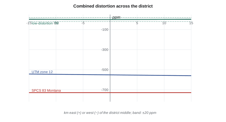
UTM zone 12: grid scale k = 0.99960618, combined factor = 0.99944877 (-551.2 ppm)
  a 2500.000 m ground distance is 2498.622 m on the grid (difference -1378 mm)

SPCS 83 Montana: grid scale k = 0.99942969, combined factor = 0.99927231 (-727.7 ppm)
  a 2500.000 m ground distance is 2498.181 m on the grid (difference -1819 mm)

Low-distortion TM: central meridian 111.3 W, k0 = 1.000158
combined-factor distortion (ppm) across the district:
                   -15 km      -8 km      +0 km      +8 km     +15 km
  h =  975 m         +8.3       +6.3       +5.5       +6.3       +8.3
  h = 1010 m         +2.8       +0.8       +0.0       +0.8       +2.8
  h = 1045 m         -2.7       -4.7       -5.5       -4.7       -2.7

At CR1 the UTM combined factor is 0.99944877, or −551 ppm, and the Montana state plane combined factor is 0.99927231, or −728 ppm. A 2,500.000 m ground distance is 2,498.181 m on the state plane grid, 1.82 m shorter, and 2,498.622 m on UTM. A contractor who staked a 2.5 km canal alignment from state plane grid distances with a total station would place the far end 1.8 m (6.0 ft) from where the design intended. Both scale and height contribute, and neither a statewide projection nor UTM can remove the height effect, which depends on local terrain.

Ground coordinates and their dangers

A common response to the grid-ground problem has been to create 'ground coordinates' by dividing grid coordinates by a project CSF, usually about a chosen point. Distances between the scaled coordinates then match ground distances near that point. The method works for a small site, but it creates a coordinate system with no formal definition: the scaled coordinates look like grid coordinates, differ from them by tens of meters or more, and cannot be converted back without knowing the exact factor and point used. Data from such systems are a frequent source of errors when projects are combined, when files are passed to GIS staff and when the project is revisited years later. If scaled coordinates are used at all, they should be given unmistakably different values, for example by subtracting large constants, and their definition should be recorded on every drawing.

Low-distortion projections

A better solution is a properly defined projection designed so that its combined factor is close to one over the project area: a low-distortion projection (LDP). An LDP is an ordinary conformal projection, usually transverse Mercator, Lambert conformal conic, oblique Mercator or oblique stereographic, chosen and parameterized for the site. Its central scale factor is set slightly greater than one to cancel the elevation factor at the project's mean ellipsoidal height \(h_0\):

and its central line or point is placed through the project. Because it is a real projection with an EPSG-style definition, it can be entered in any GIS or survey software, converted to and from latitude and longitude exactly, and documented once for all users. The design steps are: decide the acceptable distortion, often ±20 ppm (2 cm per kilometer, roughly the precision of a good total station distance); choose a projection type whose distortion pattern follows the project's shape; set the central meridian or origin near the project's center; set \(k_0\) from the mean height; then map the combined distortion over a terrain model of the area and adjust. Because distortion from height changes by about 1 ppm for every 6.4 m of relief, the achievable distortion is usually limited by the terrain, not by the projection.

For the district, a TM with central meridian 111.3° W and \(k_0 = 1.000158\) holds the combined distortion within ±6 ppm over the 30 km width of the district and a ±35 m range of heights, as the code's table shows. Projection distortion contributes only 3 ppm at 15 km from the central meridian; most of the variation comes from height. Leah defined this projection as the district's construction grid, gave it a false easting and northing that make its coordinates obviously different from state plane and UTM, and published its definition with the data standard.

Low-distortion projections are now common in the United States. Oregon's statewide system of LDP zones, Wisconsin's county coordinate systems, county systems in Minnesota and Iowa, and the low-distortion layers of SPCS2022 make the approach routine, and Montana's surveyors have used project LDPs for highway and canal work for years. Whatever the jurisdiction, an LDP should be registered with the project records, and coordinates in it should always be accompanied by their definition.