
GEOM-340 · Lesson 12 of 12 · 22 min
Practical problems
The district's canal rehabilitation went to construction in the spring after Leah's course, and the questions that came back from the field were the practical ones the course had been built to answer. This lesson works through them: a control traverse along Lateral 7 between two GNSS points, the staking of the new turnouts, the 1958 drawings, a contractor's machine-control model, a set of old and new GNSS observations, a landowner's area dispute and the bearing note on a plan. Each problem draws on several earlier lessons, and together they form a checklist for any project that uses projected coordinates.
Problem 1: a traverse between GNSS control points
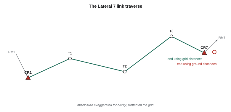
Grant's crew ran a link traverse along Lateral 7 from CR1 to CR7, 3.4 km (11,000 ft) away, both with SPCS 83 Montana coordinates on NAD83(2011) from GNSS. They measured angles and horizontal ground distances with a total station, and the backsight and foresight azimuths came from GNSS-derived reference marks at each end, so they are already grid azimuths. The traverse closes on the angles to a tenth of a second, but its position misclosure depends entirely on whether the ground distances are converted to grid distances.
import math
# A link traverse along Lateral 7 between two GNSS control points with grid coordinates
# (SPCS 83 Montana, NAD83(2011), international feet). Field data: angles right (deg)
# and horizontal ground distances (ft).
CSF = 0.99927231                    # combined factor at the project (lesson 8)
A = (1524450.751, 1192102.008)     # CR1, start
B = (1535430.293, 1192794.433)     # CR7, end of Lateral 7
az_in = 200.0                       # grid azimuth of the line from mark RM1 to CR1
az_out = 315.0                      # grid azimuth of the line from CR7 to mark RM7
legs = [(58.39989, 2666.65), (197.69991, 3436.22), (155.19961, 3069.49), (211.40046, 2102.59)]
closing_angle = 32.30010            # angle right at CR7 from the last station to RM7

# 1. Angular check
az = az_in
for ang, d in legs: az = (az + ang + 180.0) % 360.0
az_end = (az + closing_angle + 180.0) % 360.0
ang_mis = (az_end - az_out) * 3600
print(f"angular misclosure {ang_mis:+.1f} arc seconds over {len(legs) + 1} angles")
corr = -ang_mis / (len(legs) + 1) / 3600

def run(scale, label, adjust_angles=True):
    az = az_in; E, N = A; total = 0.0; path = []
    for i, (ang, d) in enumerate(legs, 1):
        az = (az + ang + (corr if adjust_angles else 0.0) + 180.0) % 360.0
        dg = d * scale; total += d
        E += dg * math.sin(math.radians(az)); N += dg * math.cos(math.radians(az)); path.append((E, N, az))
    dE, dN = E - B[0], N - B[1]; mis = math.hypot(dE, dN)
    print(f"{label:32s} misclosure dE {dE:+6.2f} ft  dN {dN:+5.2f} ft  "
          f"total {mis:5.2f} ft = 1 : {total / mis:,.0f}")
    return dE, dN, total, path

run(1.0, "ground distances used as grid")
dE, dN, total, path = run(CSF, "distances x combined factor")

# 2. Compass-rule adjustment of the scaled traverse
cum = 0.0
print("\nadjusted stations (compass rule):")
for i, ((ang, d), (E, N, az)) in enumerate(zip(legs, path), 1):
    cum += d; k = cum / total
    name = f"T{i}" if i < len(legs) else "CR7"
    print(f"  {name:4s} E {E - dE*k:11.3f}  N {N - dN*k:12.3f}   leg grid azimuth {az:9.5f}")

# 3. Staking: a design grid distance has to be laid out on the ground
grid_d = 500.00
print(f"\nto stake a {grid_d:.2f} ft grid distance, measure {grid_d / CSF:.2f} ft on the ground")angular misclosure -0.1 arc seconds over 5 angles ground distances used as grid misclosure dE +8.00 ft dN +0.55 ft total 8.02 ft = 1 : 1,406 distances x combined factor misclosure dE +0.00 ft dN +0.05 ft total 0.05 ft = 1 : 228,774 adjusted stations (compass rule): T1 E 1527061.033 N 1192637.815 leg grid azimuth 78.39990 T2 E 1530475.310 N 1192272.931 leg grid azimuth 96.09981 T3 E 1533380.636 N 1193256.348 leg grid azimuth 71.29943 CR7 E 1535430.293 N 1192794.433 leg grid azimuth 102.69989 to stake a 500.00 ft grid distance, measure 500.36 ft on the ground
Using the ground distances as if they were grid distances, the traverse misses CR7 by 8.02 ft, a closure of 1 part in 1,406, which would fail any survey standard and might send the crew back to remeasure. Multiplying each distance by the combined factor of 0.99927231 from lesson 8 reduces the misclosure to 0.05 ft, 1 part in 229,000, entirely consistent with the instrument. The 'error' of 8 ft was the 728 ppm difference between ground and grid over 11,275 ft of traverse. A closed loop traverse would not have revealed it, because a uniform scale error cancels around a loop; only a traverse between control points, or a check against GNSS, exposes it. The compass-rule adjustment then distributes the 0.05 ft along the traverse in proportion to distance and gives final grid coordinates for the intermediate stations.
Problem 2: staking from grid coordinates
The new turnouts were designed in state plane coordinates, and the contractor staked them by total station from the traverse stations. A design grid distance must be divided by the combined factor to give the distance to lay out on the ground: a 500.00 ft grid distance becomes 500.36 ft on the ground. Over the 400 ft typical of turnout staking the difference is 0.29 ft, far larger than the construction tolerance of ±0.08 ft for the turnout boxes. For the canal's structures, the project instead used the district's low-distortion projection of lesson 8, whose combined factor at the site is within a few ppm of one, so that grid and ground distances agree to a few thousandths of a foot over the same distance and the crew could stake without corrections. Converting the design from state plane to the LDP was a single, documented conversion of the whole model.
Problem 3: the 1958 drawings
The 1958 as-built drawings, georeferenced in GEOM-330 to the orthophotos with an RMS of 0.10 m on the control points but a check-point accuracy of only 1.9 m, raised a sharper question during design: where exactly are the old structures' foundations? The drawings carried coordinates on a local grid tied to two NAD27 monuments. Leah recovered one of the monuments, transformed its published NAD27 position with the national grid shift of lesson 9, and compared it with a new GNSS position: they agreed within 0.3 m, the expected accuracy of the grid for that area. The second monument was gone. With one control point, a known rotation from the drawing's bearing note and the drawing's stated scale, she defined a two-dimensional similarity transformation from the local grid to the project CRS and checked it on three surviving structures found by excavation. The residuals were 0.2 to 0.4 m. That was good enough to locate the foundations for excavation but not for design of connections to them, which were surveyed directly once exposed.
Problem 4: a contractor's machine-control model
The earthwork contractor's machine-control system needed the design surface in its own format, with a coordinate system loaded in each machine's GNSS receiver. The first model delivered showed the canal grade 0.3 % steeper than designed over a test section. The cause was a site calibration in the receivers, fitted by the contractor's technician to four control points but computed with a scale factor left free, which absorbed the 140 to 160 ppm height effect differently from the design software. The cure was to load the district's LDP definition into the receivers, with the published geoid model for heights, and to check the receivers on control before each shift. The same model then agreed with the design surface within 15 mm. The lesson is that the coordinate system is part of the design, not a setting left to whoever operates the equipment.
Problem 5: observations from different epochs
For deformation monitoring of the embankments, the engineer compared new GNSS positions of settlement monuments with positions from a survey in 2014. The raw differences showed every monument moving 9 to 11 mm south-east, including two on bedrock that could not have moved. The 2014 coordinates had been computed in a different NAD83 realization and epoch from the new ones. Bringing both sets to NAD83(2011) epoch 2010.00 with NGS's tools removed the common shift, and the remaining differences, a few millimeters of settlement on the fill sections only, were real. Monitoring always compares like with like: same frame, same realization, same epoch, same processing.
Problem 6: an area dispute
A landowner disputed the district's water assessment because the GIS area of his field, 62.50 ha (154.4 acres), was larger than the 62.40 ha (154.2 acres) on his deed. Leah's analysis had three parts. The GIS area was a grid area on state plane; converting it to the ellipsoid with the scale factor of lesson 2 gave 62.57 ha. The deed area came from a survey on the ground; the field boundary in the GIS was digitized from an orthophoto and included 0.20 ha of the ditch right-of-way that the deed excluded. Corrected for both, the GIS area was 62.37 ha, close to the deed area. The district changed its assessment calculation to use ellipsoidal areas of the parcel fabric, not grid areas of digitized fields.
Problem 7: the bearing note
Every plan the district issues now carries a note stating the basis of bearings, for example: 'Bearings are grid bearings on SPCS 83 Montana (2500), NAD83(2011) epoch 2010.00, derived from GNSS observations at CR1 and CR7. Grid convergence at CR1 is −1°18'54\"; to obtain true bearings add the convergence.' Without such a note, a bearing of N 88° E on a plan could be true, grid on state plane, grid on UTM or magnetic, and the four can differ by about 10° or more once magnetic declination is included. The note also gives distances as grid or ground, and the combined factor used.
A checklist for projected coordinates
| Question | Where in the course |
|---|---|
| What datum, realization or version, and epoch? | Lessons 9 and 10 |
| What projection, with which parameters, units and axis order? | Lessons 3 to 7 and 11 |
| Are distances grid, ellipsoid or ground, and what combined factor applies? | Lesson 8 |
| Are bearings grid, true or magnetic, and what is the convergence? | Lessons 4 and 6 |
| Are heights ellipsoidal or orthometric, on which datum and geoid model? | Lessons 8 and 10, and Geodesy I |
| Which transformation was used between datums, and was it tested on control? | Lessons 9 and 11 |
| Is a low-distortion projection better for construction? | Lesson 8 |
| Is everything recorded in the metadata and on the drawings? | All lessons |
The district adopted the checklist as part of its data standard. Leah's closing advice to the course was that projections and datums are not obstacles but tools: once the system of every coordinate is stated and the corrections between systems are understood, data from 1958 drawings, provincial or state databases, GNSS receivers and contractors' machines can be combined to whatever accuracy the data themselves allow. The errors in practice come almost never from the formulas, which software computes to nanometers, and almost always from missing information about which formulas were used.
Worked problem
Combined factor misclosure check
A link traverse of total length 11,275 ft between two GNSS points misses the end point by 8.0 ft when ground distances are used. The project's combined factor is 0.99927. Is the misclosure explained by the factor?
Show solution
- \[\delta = L\,(1 - \text{CSF}) = 11{,}275 \times 0.00073 = 8.2 \text{ ft}\]
Answer: Almost all of it. The traverse runs roughly in a straight line, so the scale error accumulates along its direction. Recompute with grid distances; what remains is the survey's true misclosure.
Worked problem
Converting a design distance for staking
A turnout is designed 388.45 ft from a traverse station along a grid line where the combined factor is 0.99927. What distance should be laid out on the ground?
Show solution
- \[s_{ground} = \frac{388.45}{0.99927} = 388.73 \text{ ft}\]
Answer: The ground distance is 0.28 ft longer than the grid distance, more than the turnout's tolerance. On the district's LDP, the same layout would need no correction.
Common mistakes
MistakeTesting traverse closure only around loops.
InsteadClose traverses on independent control to expose scale errors.
MistakeStaking grid distances directly on the ground.
InsteadDivide by the combined factor, or design in a low-distortion projection.
MistakeLeaving site calibrations to equipment operators.
InsteadDefine the coordinate system centrally and load it in every receiver.
MistakeComparing monitoring surveys made in different frames or epochs.
InsteadBring both to one frame, version and epoch first.
MistakeIssuing plans without a basis of bearings and distances.
InsteadState the CRS, the bearing basis, the convergence and whether distances are grid or ground.
Summary and key terms
- A uniform scale error cancels around a loop; link traverses between control expose it.
- Grid distances must be divided by the combined factor for staking, unless an LDP is used.
- Old drawings need datum transformations and checks on recovered features.
- Machine-control systems should use the project's defined CRS, not ad hoc calibrations.
- Monitoring compares coordinates in the same frame, version and epoch.
- Legal areas and bearings need stated bases; the checklist summarizes what every coordinate needs.
- Link traverse
- A traverse that starts and ends on different points of known coordinates.
- Compass rule
- An adjustment that distributes a traverse misclosure in proportion to distance.
- Basis of bearings
- The statement on a plan of the reference direction for its bearings.
- Machine control
- Guidance of construction equipment from a design model by GNSS or total station.
- Similarity transformation
- A transformation with translation, rotation and one scale factor.
- Deformation monitoring
- Repeated surveys to detect movement of structures or ground.
Practice problems
Work each problem on paper first, then reveal the answer to check.
Why does a closed loop not reveal a scale error?
Show answer
A uniform scale changes every leg in proportion, so the loop still closes.
A traverse closes to 1:3,000 on ground distances and 1:200,000 on grid distances. What does that indicate?
Show answer
The scale difference between ground and grid explains the misclosure; the survey is sound.
What should a basis of bearings note contain?
Show answer
The CRS with datum and epoch, the source of the bearings, the convergence and whether distances are grid or ground.
Two monitoring surveys differ by 13 mm everywhere, even on bedrock. What is the likely cause?
Show answer
Different frames, versions or epochs.
Why is an LDP useful for staking?
Show answer
Grid and ground distances agree, so no factor is needed.
Lesson quiz · 5 questions
Score 60% or more to complete this lesson.
Create a free account to save your progress, take quizzes and earn a certificate.