
GEOM-340 · Lesson 5 of 12 · 23 min
Azimuthal projections
The district's new radio system for gate telemetry needed a coverage map: circles of equal distance around the repeater on the coulee rim, with true bearings to each remote gate so that antennas could be aimed. Leah drew it on an azimuthal equidistant projection centered on the repeater, the one projection on which every straight line from the center is both a true distance and a true bearing. That map introduced the district's staff to the third family of projections, those made on a plane touching the globe at one point. Azimuthal projections are used for polar regions, for maps of distance and direction from a place, for national grids in compact countries and provinces, and in disguise inside every GNSS receiver that reports local east, north and up coordinates.
The azimuthal family
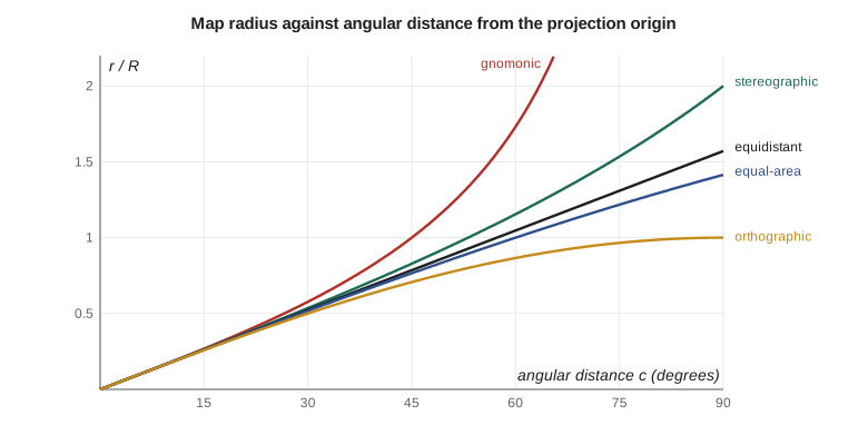
An azimuthal projection is built around a center point. Every point on the globe is described by its angular distance \(c\) from the center, measured along the great circle, and its azimuth \(\alpha\) from the center. The projection keeps the azimuth and converts the angular distance into a radius on the map:
so that all great circles through the center are straight lines and all directions from the center are true. The members of the family differ only in the radius function \(r(c)\). The scale along a radius is \(h = r'(c)/R\) and the scale at right angles to it is \(k = r(c)/(R\sin c)\), so lines of equal distortion are circles around the center. That pattern suits a compact, roughly circular region: the distortion depends only on how far a point is from the center, in whatever direction.
| Projection | Radius r(c) | Property | Distortion grows | Typical use |
|---|---|---|---|---|
| Gnomonic | R tan c | Great circles are straight lines | Very fast; limited to under 90° | Planning great-circle routes, seismology |
| Stereographic | 2R tan(c/2) | Conformal | Slowly; scale (1 + cos c)⁻¹ × 2 | Polar maps, national and provincial grids |
| Azimuthal equidistant | R c | True distance from the center | Only at right angles to radii | Range rings, radio and air routes |
| Lambert azimuthal equal-area | 2R sin(c/2) | Equal-area | Shapes stretch tangentially | Continental statistics maps |
| Orthographic | R sin c | Perspective from infinity | Rapidly near the edge | Pictures of the globe |
Perspective projections: gnomonic, stereographic, orthographic
Three members can be built literally with light. With the light at the center of the globe, each point is projected onto the tangent plane along a line through the center: this is the gnomonic projection. Every great circle lies in a plane through the center, so every great circle projects as a straight line. A straight line drawn on a gnomonic map between two places is the shortest route on the sphere, which is why navigators once used gnomonic charts to plan great-circle routes before transferring them to Mercator charts to steer. The gnomonic cannot show a whole hemisphere, and its distortion grows so fast that it is never used for measurement.
With the light at the point opposite the center, the antipode, the result is the stereographic projection, known to Hipparchus and used for star charts and astrolabes in antiquity. It is conformal, and it has a further property shared by no other projection: every circle on the globe, large or small, projects as a circle or a straight line. Its scale \(k = 2/(1 + \cos c)\) grows slowly, reaching only 1.00008 at 1° (111 km) from the center and 2 at 90°. Stereographic projections with the center at a pole are the standard for polar mapping, including the Universal Polar Stereographic (UPS) system that complements UTM north of 84° N and south of 80° S. Oblique stereographic projections are used for national or provincial grids in compact regions: the Netherlands' national grid is an oblique stereographic, and so are the grids of New Brunswick and Prince Edward Island in Canada.
With the light at an infinite distance, the result is the orthographic projection, which looks like a photograph of the globe from space. It is neither conformal nor equal-area and is used only for illustration.
Non-perspective members: equidistant and equal-area
The azimuthal equidistant projection makes the map radius equal to the distance along the surface, \(r = Rc\). Distances and directions from the center are both true, so a ruler and protractor placed on the center give the true distance and azimuth to any point on the map. Circles of equal distance around the center are true range rings. The projection is used for radio and radar coverage, for maps of flight distances from a city, for seismic maps centered on a recording station and, in polar aspect, for the emblem of the United Nations. Distortion appears only at right angles to the radii: a circle at angular distance \(c\) is drawn with circumference \(2\pi Rc\) instead of \(2\pi R\sin c\), so at 1,000 km from the center the tangential scale is 1.004 and at 3,000 km 1.038.
Lambert's azimuthal equal-area projection of 1772, with \(r = 2R\sin(c/2)\), compresses the radii exactly as much as the circles are stretched, keeping areas true. It is a good projection for maps of continents or oceans where area matters: the European Union uses it for its statistical grid, and it has been used for maps of North America, centered near 45° N and 100° W, in national atlases. For a region the size of a province or state, an equal-area conic is usually chosen instead because its distortion pattern suits a band of latitude.
Ellipsoidal forms and local planes
The formulas above are for a sphere. For the ellipsoid, conformal azimuthal projections are usually made in two steps: the ellipsoid is first mapped conformally onto a sphere that fits it closely near the center, the 'conformal sphere', and the sphere is then projected stereographically. This 'double stereographic' method is used by New Brunswick's grid and by the Netherlands. The azimuthal equidistant and equal-area projections have ellipsoidal forms based on geodesics and authalic (equal-area) latitudes. Software handles these details; the user's task is to choose the right method name, because 'Oblique Stereographic' and 'Polar Stereographic' are separate methods in the EPSG registry, each with variants.
A local tangent plane is the azimuthal idea at its simplest. Geodesy I converted ECEF coordinates into local east, north and up (ENU) coordinates at a point: these are coordinates on a plane tangent to the ellipsoid at the origin, effectively an orthographic projection of nearby points onto that plane. Over a few kilometers ENU coordinates and a stereographic projection centered at the same point agree to millimeters, and both have distortion of only a part per million or two at 15 km. Construction layout software that 'localizes' GNSS observations to a site often uses a tangent plane or stereographic projection of this kind, with a scale factor set to match the ground, which lesson 8 discusses.
import math
R = 6371000.0

# The four classic azimuthal projections on a sphere, around the point (lat0, lon0).
# Each one keeps azimuths from the origin true and differs only in how the
# angular distance c from the origin becomes a radius r on the map.
radius = {
    "gnomonic":       lambda c: R * math.tan(c),
    "stereographic":  lambda c: 2 * R * math.tan(c / 2),
    "equidistant":    lambda c: R * c,
    "equal-area":     lambda c: 2 * R * math.sin(c / 2),
    "orthographic":   lambda c: R * math.sin(c),
}
def scales(name, c):
    """Radial scale h and tangential scale k at angular distance c."""
    d = 1e-7
    h = (radius[name](c + d) - radius[name](c)) / (R * d)
    k = radius[name](c) / (R * math.sin(c))
    return h, k

def az_dist(lat0, lon0, lat, lon):
    """Spherical azimuth (deg) and angular distance (rad) from the origin."""
    p0, p, dl = math.radians(lat0), math.radians(lat), math.radians(lon - lon0)
    c = math.acos(math.sin(p0)*math.sin(p) + math.cos(p0)*math.cos(p)*math.cos(dl))
    az = math.atan2(math.sin(dl)*math.cos(p), math.cos(p0)*math.sin(p) - math.sin(p0)*math.cos(p)*math.cos(dl))
    return math.degrees(az) % 360, c

print(f"{'distance from origin':22s}" + "".join(f"{n:>16s}" for n in radius))
for km in (15, 100, 500, 1000, 3000):
    c = km * 1000 / R
    row = ""
    for n in radius:
        h, k = scales(n, c)
        row += f"   h{h:6.4f} k{k:6.4f}"[-16:]
    print(f"{km:8d} km            " + row)

# Range rings for the district's radio repeater: azimuthal equidistant around CR1
lat0, lon0 = 47.50600422, -111.29779092
sites = {"Helena": (46.59, -112.04), "Billings": (45.78, -108.50), "Lethbridge": (49.70, -112.83)}
print("\nAzimuthal equidistant around CR1 (distances and azimuths are true from the origin)")
for s, (la, lo) in sites.items():
    az, c = az_dist(lat0, lon0, la, lo)
    r = radius["equidistant"](c)
    x, y = r * math.sin(math.radians(az)), r * math.cos(math.radians(az))
    print(f"  {s:13s} azimuth {az:6.2f} deg  distance {r/1000:7.2f} km  map x {x/1000:8.2f} km  y {y/1000:8.2f} km")

# A stereographic plane for the district only: how small is its distortion?
for km in (5, 10, 15, 20):
    c = km * 1000 / R; k = scales("stereographic", c)[1]
print(f"stereographic plane around the district, {km:2d} km out: k = {k:.9f} ({(k-1)*1e6:.2f} ppm)")distance from origin gnomonic stereographic equidistant equal-area orthographic
15 km h1.0000 k1.0000 h1.0000 k1.0000 h1.0000 k1.0000 h1.0000 k1.0000 h1.0000 k1.0000
100 km h1.0002 k1.0001 h1.0001 k1.0001 h1.0000 k1.0000 h1.0000 k1.0000 h0.9999 k1.0000
500 km h1.0062 k1.0031 h1.0015 k1.0015 h1.0000 k1.0010 h0.9992 k1.0008 h0.9969 k1.0000
1000 km h1.0250 k1.0124 h1.0062 k1.0062 h1.0000 k1.0041 h0.9969 k1.0031 h0.9877 k1.0000
3000 km h1.2592 k1.1221 h1.0575 k1.0575 h1.0000 k1.0379 h0.9724 k1.0284 h0.8912 k1.0000
Azimuthal equidistant around CR1 (distances and azimuths are true from the origin)
Helena azimuth 209.18 deg distance 116.35 km map x -56.72 km y -101.59 km
Billings azimuth 130.92 deg distance 287.11 km map x 216.95 km y -188.05 km
Lethbridge azimuth 335.78 deg distance 268.70 km map x -110.22 km y 245.06 km
stereographic plane around the district, 5 km out: k = 1.000000154 (0.15 ppm)
stereographic plane around the district, 10 km out: k = 1.000000616 (0.62 ppm)
stereographic plane around the district, 15 km out: k = 1.000001386 (1.39 ppm)
stereographic plane around the district, 20 km out: k = 1.000002464 (2.46 ppm)The first table shows how the five radius functions behave. At 15 km from the center all of them are indistinguishable from the truth at four decimal places. At 500 km the stereographic scale is 1.0015 in every direction, the equidistant radial scale is exactly 1 with tangential scale 1.0010, and the gnomonic radial scale is already 1.0062. At 3,000 km the gnomonic radial scale is 1.26. The second part centers an azimuthal equidistant projection on CR1: Helena lies at azimuth 209.18° and 116.35 km, Billings at 130.92° and 287.11 km, and Lethbridge at 335.78° and 268.70 km. These are true spherical distances and azimuths, good to a few tenths of a percent; for antenna aiming that is ample, and for surveying the geodesic calculations of Geodesy I would be used instead. The last lines show that a stereographic plane centered on the district has a distortion of 1.4 ppm at 15 km, which is negligible compared with the height effect of 160 ppm discussed in lesson 8.
Choosing an azimuthal projection
The choice within the family follows the purpose. For a map that must show true distances and directions from one place, use the azimuthal equidistant. For a compact region that needs conformal coordinates, such as a small province, an island or a site, use the stereographic. For an equal-area map of a continent or ocean, use the Lambert azimuthal equal-area. For a polar region, use a polar stereographic for conformal work or a polar Lambert equal-area for statistics. And for planning shortest routes over long distances, the gnomonic shows them as straight lines. The repeater coverage map used the azimuthal equidistant; the district's construction site plans could equally well have used an oblique stereographic, and lesson 8 compares that choice with a transverse Mercator low-distortion projection.
Worked problem
Scale of a stereographic projection
A stereographic projection is centered on a project with \(k_0 = 1\). What is the scale factor 25 km from the center on a sphere of radius 6,371 km?
Show solution
- \[c = \frac{25}{6371} = 0.003924 \text{ rad}\]
- \[k = \frac{2}{1 + \cos c} = \frac{2}{1 + 0.9999923} = 1.0000038\]
Answer: The scale is 3.8 ppm too large at 25 km. Reducing \(k_0\) to 0.999998 would spread the error to −2 ppm at the center and +1.8 ppm at the edge.
Worked problem
Reading a coverage map
On the azimuthal equidistant projection centered on CR1, a gate at map coordinates \(x = 9.20\) km, \(y = -4.10\) km must be reached by the radio. What distance and azimuth should the antenna installer use?
Show solution
- \[r = \sqrt{9.20^2 + 4.10^2} = 10.07 \text{ km}\]
- \[\alpha = \operatorname{atan2}(9.20, -4.10) = 114.0^\circ\]
Answer: The gate is 10.07 km away at an azimuth of 114.0° from true north. Both values are true because the map is azimuthal equidistant about CR1; at 10 km the tangential distortion is under 1 ppm.
Common mistakes
MistakeMeasuring distances between two points on an azimuthal equidistant map when neither is the center.
InsteadOnly distances from the center are true; compute other distances on the ellipsoid.
MistakeUsing a gnomonic map for measurement.
InsteadIts scale grows very rapidly; use it only to show great-circle routes.
MistakeChoosing 'Polar Stereographic' for an oblique stereographic grid or the reverse.
InsteadUse the exact EPSG method name and its parameters.
MistakeTreating ENU coordinates as a projection valid over a large area.
InsteadA tangent plane is accurate only near its origin; for larger areas use a proper projection.
MistakeForgetting that azimuths from the center are true but azimuths elsewhere are not.
InsteadApply convergence and arc-to-chord corrections away from the center.
Summary and key terms
- Azimuthal projections map a plane tangent at one point; azimuths from the center are true.
- Members differ only in the radius function r(c); distortion depends only on distance from the center.
- Gnomonic: great circles straight. Stereographic: conformal, circles stay circles. Orthographic: a view of the globe.
- Azimuthal equidistant: true distance and direction from the center; used for range rings.
- Lambert azimuthal equal-area: true areas, used for continents and statistical grids.
- Oblique and double stereographic projections serve compact regions; polar stereographic serves the poles.
- Azimuthal projection
- A projection onto a plane at one point, keeping azimuths from that point true.
- Gnomonic projection
- The azimuthal projection from the globe's center; great circles are straight lines.
- Stereographic projection
- The conformal azimuthal projection from the antipode of the center.
- Azimuthal equidistant
- The azimuthal projection keeping true distances from the center.
- Double stereographic
- A conformal mapping of the ellipsoid to a sphere followed by a stereographic projection.
- UPS
- Universal Polar Stereographic, the grid for the polar caps beyond UTM.
- Local tangent plane
- East, north and up coordinates on a plane touching the ellipsoid at an origin.
Practice problems
Work each problem on paper first, then reveal the answer to check.
What is the stereographic scale factor 90° from the center?
Show answer
2/(1 + cos 90°) = 2.
Which azimuthal projection would show the shortest air route from Calgary to Tokyo as a straight line?
Show answer
The gnomonic.
On an azimuthal equidistant map, what is the tangential scale at angular distance c?
Show answer
c / sin c.
Why do compact provinces and countries use oblique stereographic grids?
Show answer
Distortion depends only on distance from the center, and the projection is conformal.
Which azimuthal projection would you use for an equal-area map of the Arctic Ocean?
Show answer
A polar Lambert azimuthal equal-area.
Lesson quiz · 5 questions
Score 60% or more to complete this lesson.
Create a free account to save your progress, take quizzes and earn a certificate.