Managed portfolios, performance evaluation, regulation and capstone

Most people invest through someone else: a mutual fund, an exchange-traded fund, a pension plan or an adviser. This final lesson looks at managed portfolios from the client's side. It compares the main fund structures, shows how much fees cost over a lifetime, reviews the evidence on active and passive management, and explains the measures used to judge whether a manager has added value after accounting for risk. It then summarizes how investors are protected by regulation and professional standards, and closes with a capstone that brings the course together: building and evaluating a portfolio for an invented investor. As throughout the course, this is education, not personal investment advice.

Fund structures

A mutual fund pools investors' money and issues units or shares that are bought and redeemed at the fund's net asset value (NAV), calculated once a day. An exchange-traded fund (ETF) also pools assets, but its units trade on an exchange throughout the day, and authorized dealers create and redeem units in large blocks, which keeps the market price close to NAV. Most ETFs track an index, though actively managed ETFs have grown quickly. Closed-end funds issue a fixed number of shares that trade on an exchange, often at a discount or premium to NAV. Hedge funds are private, lightly regulated pools for wealthy and institutional investors that use leverage, short selling and derivatives, typically charging a management fee plus a share of profits. Segregated funds (in Canada) and variable annuities (in the United States) wrap funds in insurance contracts with guarantees, at extra cost.

US mutual funds and ETFs are registered with the SEC under the Investment Company Act of 1940, which limits leverage and requires daily pricing, independent directors and disclosure in a prospectus and summary prospectus, including the expense ratio. Funds may charge 12b-1 distribution fees and sales loads, which are disclosed in a fee table. Since the SEC's 2019 ETF rule, most ETFs can launch without individual exemptions.

The cost of fees

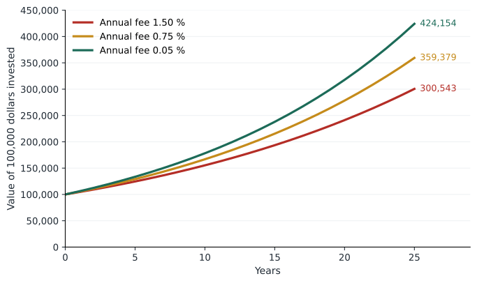
Fees come straight out of returns, every year, whatever the fund's performance, and they compound. A difference of one or two percentage points a year looks small but grows into a large share of ending wealth over a working life. Fees are expressed as an annual percentage of assets: the management expense ratio in Canada, or expense ratio in the United States, covers management, administration and, for many funds, advice or trailing commissions. Trading costs inside the fund are additional and are reported separately as a trading expense ratio.

US fees are among the lowest in the world. The Investment Company Institute reported asset-weighted average expense ratios for 2025 of about 0.40 % for equity mutual funds, 0.36 % for bond mutual funds and 0.14 % for index equity ETFs; some broad index funds charge only a few hundredths of a percentage point. Investors who pay for advice usually pay an additional advisory fee, often around 1 % a year.

Active versus passive management

An active manager tries to beat a benchmark by selecting securities or timing the market; a passive manager tries to match it at low cost. William Sharpe's arithmetic of active management, published in 1991, explains why active managers as a group must lag: before costs, the average actively managed dollar must earn the market return, because active and passive investors together hold the market and passive investors earn exactly the market. After costs, the average active dollar must therefore earn less. Some managers will beat the market, but identifying them in advance is hard, and past winners have rarely kept winning.

S&P Dow Jones Indices' SPIVA scorecards have repeatedly found that a large majority of US equity funds trail their benchmarks over long periods; 79 % of active large-cap funds underperformed the S&P 500 in 2025, and at least 80 % of equity funds underperformed over the ten years to 2025. Morningstar's research has also found that the expense ratio is one of the most reliable predictors of a fund's future relative performance.

These results do not prove markets are perfectly efficient: costs, career pressures and the difficulty of the task can explain them. Nor do they say active management has no place. Some investors value features that index funds lack, and in less efficient markets, such as small companies or some bond sectors, active managers may have more room. But the evidence explains the rapid growth of index funds and ETFs in both countries, and it puts the burden of proof on anyone charging higher fees.

Measuring risk-adjusted performance

Raw returns are not enough to judge a manager, because a manager can beat a benchmark simply by taking more risk. Four classic measures adjust for risk in different ways. The Sharpe ratio divides excess return by the standard deviation; it suits an investor whose whole portfolio is the fund. The Treynor ratio divides excess return by beta; it suits a fund that is one part of a diversified portfolio, where only systematic risk matters. Jensen's alpha is the return in excess of what the CAPM predicts for the fund's beta, the intercept of the regression in lesson 6; a multifactor version, from lesson 7, adjusts for size, value and momentum exposures. The information ratio divides alpha, or the return over the benchmark, by the tracking error, the standard deviation of the difference; it measures the consistency of a manager's value added. M², or Modigliani risk-adjusted performance, scales the fund to the market's volatility using the risk-free asset and reports the resulting return, which is easier to interpret than a ratio.

# Performance measures on seeded simulated monthly returns
import numpy as np
rng = np.random.default_rng(12)
months = 120
rf = np.full(months, 0.025 / 12)
mkt = rf + rng.normal(0.006, 0.045, months)
fund = rf + 0.0008 + 0.9 * (mkt - rf) + rng.normal(0, 0.015, months)   # small true alpha

def annual(x): return x.mean() * 12
ex_f, ex_m = fund - rf, mkt - rf
beta = np.cov(ex_f, ex_m)[0, 1] / ex_m.var(ddof=1)
alpha = annual(ex_f) - beta * annual(ex_m)
resid = ex_f - beta * ex_m
sharpe_f = annual(ex_f) / (fund.std(ddof=1) * np.sqrt(12))
sharpe_m = annual(ex_m) / (mkt.std(ddof=1) * np.sqrt(12))
treynor = annual(ex_f) / beta
info = alpha / (resid.std(ddof=1) * np.sqrt(12))
m2 = annual(rf) + sharpe_f * mkt.std(ddof=1) * np.sqrt(12)
t_alpha = (resid.mean() / (resid.std(ddof=1) / np.sqrt(months)))
print(f"beta {beta:.2f}  annual alpha {alpha:+.2%} (t = {t_alpha:.2f})")
print(f"Sharpe: fund {sharpe_f:.2f}, market {sharpe_m:.2f}   Treynor {treynor:.2%}")
print(f"information ratio {info:.2f}   M-squared {m2:.2%} vs market {annual(mkt):.2%}")

beta 0.85  annual alpha +1.21% (t = 0.78)
Sharpe: fund 0.69, market 0.65   Treynor 10.80%
information ratio 0.25   M-squared 12.53% vs market 11.87%

The simulation shows how hard it is to prove skill statistically. The fund was built with a true alpha of almost 1 % a year, yet after ten years of monthly data the t-statistic is unlikely to clear the conventional level of 2. With realistic levels of noise, it can take decades to separate a skilled manager from a lucky one, which is why investors should look at the process and costs behind a track record, not just the numbers.

Pitfalls in performance data

Several biases flatter reported fund performance. Survivorship bias: funds that perform badly are often merged or closed, so averages computed only from surviving funds overstate what investors actually earned. Benchmark choice: a manager who holds small companies but is measured against a large-company index can appear skilled in years when small companies do well. Backfill bias in hedge fund databases: funds report only after a good start. And time period: almost any strategy has looked good over some period. Performance attribution helps by splitting a portfolio's return relative to its benchmark into an allocation effect, from over- or under-weighting asset classes or sectors, and a selection effect, from picking better or worse securities within them.

Regulation and investor protection

US securities regulation is led by the SEC, with FINRA overseeing broker-dealers and state regulators overseeing smaller investment advisers. Broker-dealers must act in the customer's best interest under Regulation Best Interest, and registered investment advisers owe a fiduciary duty. If a member brokerage firm fails, the Securities Investor Protection Corporation (SIPC) protects customer securities and cash up to $500,000, including up to $250,000 in cash. It does not protect against market losses. Disputes with brokers usually go to FINRA arbitration.

Professional standards complement regulation. The CFA Institute's Code of Ethics and Standards of Professional Conduct, which charterholders in both countries must follow, require putting clients' interests first, exercising independent judgment, disclosing conflicts, dealing fairly and presenting performance accurately, including under the Global Investment Performance Standards described in lesson 3.

Capstone: building and evaluating a portfolio

Maya is 35, lives in Ohio, earns $95,000 a year and has $60,000 to invest for retirement, with access to a 401(k) with an employer match and room in a Roth IRA. She has an emergency fund, a long horizon and, by questionnaire and discussion, moderate risk aversion (A ≈ 3). She wants low costs and broad diversification. This invented case shows how the course's tools fit together; it is not advice for any real person.

Step 1, capital market assumptions: use the illustrative four-asset inputs from lesson 5, with a risk-free rate of 3 %. Step 2, the risky portfolio: the long-only tangency portfolio from lesson 5 holds roughly 12 % Canadian shares, 22 % US shares, 8 % international shares and 58 % bonds, with an expected return near 5.9 % and a standard deviation near 8.3 %. Step 3, the allocation: with A = 3, the optimal fraction in the risky portfolio is y* = (0.059 − 0.03) ÷ (3 × 0.083²), about 1.4, which would mean borrowing. Maya prefers not to use leverage, so she holds 100 % in the risky portfolio and tilts it toward shares, choosing a simpler 65 % equity and 35 % bond mix, spread across the three equity regions roughly in proportion to world market values with a modest home weighting. Step 4, implementation: three or four broad index ETFs with low fees. Step 5, location and accounts, set out below. Step 6, monitoring: rebalance annually or when any weight drifts more than five percentage points, and review the plan when her circumstances change.

For location, Maya first contributes enough to her 401(k) to receive the full employer match, an immediate return no investment can beat, holding bond funds there to shelter fully taxed interest. She then funds her Roth IRA with equity index funds, where tax-free growth is most valuable, and returns to the 401(k) with any remaining savings. If she later invests in a taxable account, broad equity ETFs, which generate mostly qualified dividends and long-term gains, are the natural candidates.

# Monte Carlo projection of Maya's 65/35 plan (illustrative inputs, education only)
import numpy as np
rng = np.random.default_rng(2026)
years, sims = 30, 20000
mu, sigma, cost = 0.067, 0.11, 0.002
r = rng.normal(mu - cost, sigma, (sims, years))
wealth = np.full(sims, 60_000.0)
for t in range(years):
    wealth = wealth * (1 + r[:, t]) + 6_000
p5, p50, p95 = np.percentile(wealth, [5, 50, 95])
print(f"median ${p50:,.0f}; 5th percentile ${p5:,.0f}; 95th percentile ${p95:,.0f}")
print(f"chance of ending below $500,000: {np.mean(wealth < 500_000):.1%}")
print(f"median in today's dollars at 2 % inflation: ${p50 / 1.02**30:,.0f}")

median $824,051; 5th percentile $397,409; 95th percentile $1,746,780
chance of ending below $500,000: 13.2%
median in today's dollars at 2 % inflation: $454,935

Every step uses tools from the course: utility and risk aversion from lesson 4, the efficient frontier from lesson 5, the CAPM and factor thinking from lessons 6 and 7 to decide that low-cost index exposure is a sensible core, bond duration from lesson 10 to choose the bond fund's maturity, taxes and accounts from lesson 2, risk measures from lesson 3, and fees and performance evaluation from this lesson to monitor the result. The portfolio is not optimal in any precise sense; it is a reasoned, diversified, low-cost plan that Maya understands and can stick with through bad markets, which is often the most important feature of all.