
FIN-301 · Lesson 6 of 12 · 25 min
The capital asset pricing model
Lessons 4 and 5 told an individual investor how to build the best portfolio given their forecasts. The capital asset pricing model (CAPM), developed in the 1960s by William Sharpe, John Lintner and Jan Mossin, asks what happens if every investor does this. Its answer is the most famous equation in finance: an asset's expected return depends only on its beta, its sensitivity to the market portfolio. FIN-201 lesson 10 used the CAPM to estimate the cost of equity. This lesson shows where the model comes from, how the capital market line and the security market line differ, how beta is estimated in practice and with what error, and what decades of testing say about whether the model works.
Assumptions
The CAPM rests on strong simplifying assumptions. Investors are price takers who care only about the mean and variance of returns over a single common horizon. They can borrow and lend any amount at the same risk-free rate, hold any fraction of any traded asset and sell short without limit. There are no taxes or transaction costs. And, crucially, investors agree on the expected returns, variances and covariances of all assets: they have homogeneous expectations. None of these is literally true, but the model's purpose is to show the logic of pricing in a well-functioning market, and many of its conclusions survive when assumptions are relaxed.
From the market portfolio to the capital market line
If every investor has the same inputs, every investor computes the same tangency portfolio from lesson 5. Since all investors hold risky assets in those same proportions, and every share must be held by someone, the tangency portfolio must be the market portfolio: all risky assets weighted by their market values. The capital allocation line through the market portfolio is called the capital market line (CML). It describes the best risk–return combinations available to any investor, and its slope is the market Sharpe ratio. The model thus gives a theoretical basis for passive investing: a market-capitalization-weighted index fund combined with treasury bills is an efficient portfolio.
The CML applies only to efficient portfolios. A single share, which carries diversifiable risk, lies below it. To price individual assets, we need to know how much each contributes to the risk of the market portfolio, and that is measured by beta.
The security market line
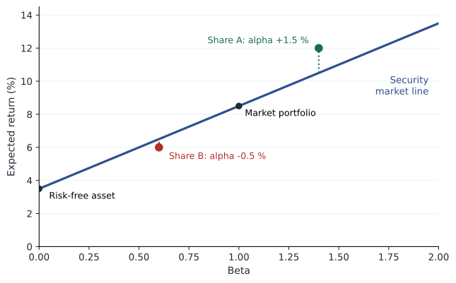
An asset's contribution to the market portfolio's variance is proportional to its covariance with the market. Scaled by the market variance, that contribution is beta. In equilibrium, every asset must offer the same reward per unit of contribution to market risk, otherwise investors would shift money and change prices until it did. The result is the security market line (SML): an asset's expected return equals the risk-free rate plus its beta times the market risk premium.
The market has a beta of 1 by definition, and the risk-free asset a beta of 0. A share with a beta of 1.5 tends to move 1.5 % for each 1 % move in the market and must offer one and a half times the market risk premium. Beta is additive: a portfolio's beta is the weighted average of its holdings' betas. Note the contrast with the CML, which uses total risk (standard deviation) and applies only to efficient portfolios; the SML uses beta and applies to every asset and portfolio.
Alpha
The difference between an asset's expected return, as forecast by an analyst, and the return the SML requires for its beta is its alpha. A positive alpha means the asset offers more than fair compensation for its systematic risk, so it appears underpriced; investors who agree will buy it, pushing its price up until the alpha disappears. In the CAPM's equilibrium, all alphas are zero. In practice, analysts hunt for alphas, and fund managers are judged on the alpha they deliver after adjusting for beta, as lesson 12 explains.
Worked problem
Using the SML to find alpha
The risk-free rate is 3.5 % and the expected market return is 8.5 %. An analyst forecasts a 12 % return on a share with beta 1.4 and a 6 % return on a share with beta 0.6. Which looks underpriced?
Show solution
- Market risk premium = 5 %.
- Required return, share A: 3.5 + 1.4 × 5 = 10.5 %. Alpha = 12 − 10.5 = +1.5 %.
- Required return, share B: 3.5 + 0.6 × 5 = 6.5 %. Alpha = 6 − 6.5 = −0.5 %.
Answer: Share A plots above the SML and looks underpriced; share B plots below and looks overpriced, if the analyst's forecasts are right.
Estimating beta
Beta is not observed; it is estimated, usually by regressing a share's excess returns on the market's excess returns over a past period. The slope of that regression, called the characteristic line, is the estimated beta, the intercept is the historical alpha, and the scatter around the line measures firm-specific risk. Common choices are five years of monthly returns or two years of weekly returns. The choices matter: different periods, return frequencies and market indices give different betas, which is why published betas for the same company often disagree.
For a US share, the usual market index is the S&P 500, a broad proxy for US equities. For companies with large foreign operations or investors, some analysts prefer a global index such as the MSCI All Country World Index. Betas measured against the S&P 500 and against a world index can differ noticeably.
# Estimating beta by regression on seeded simulated monthly excess returns
import numpy as np
rng = np.random.default_rng(6)
months = 60
market = rng.normal(0.005, 0.045, months)           # market excess returns
true_beta, true_alpha = 1.3, 0.0
stock = true_alpha + true_beta * market + rng.normal(0, 0.06, months)

X = np.column_stack([np.ones(months), market])
coef, res, *_ = np.linalg.lstsq(X, stock, rcond=None)
alpha, beta = coef
resid = stock - X @ coef
s2 = resid @ resid / (months - 2)
se_beta = np.sqrt(s2 / ((market - market.mean()) @ (market - market.mean())))
r2 = 1 - resid @ resid / ((stock - stock.mean()) @ (stock - stock.mean()))
print(f"estimated beta {beta:.3f}  (standard error {se_beta:.3f})")
print(f"95 % confidence interval {beta - 1.96 * se_beta:.2f} to {beta + 1.96 * se_beta:.2f}")
print(f"monthly alpha {alpha:.4f}   R-squared {r2:.2f}")
print(f"adjusted (Blume) beta: {2/3 * beta + 1/3:.3f}")

# Same stock, different 5-year windows: how much does the estimate move?
estimates = []
for _ in range(5):
    m = rng.normal(0.005, 0.045, months)
    s = true_beta * m + rng.normal(0, 0.06, months)
    estimates.append(np.polyfit(m, s, 1)[0])
print("betas from five other windows:", " ".join(f"{b:.2f}" for b in estimates))estimated beta 1.128 (standard error 0.180) 95 % confidence interval 0.77 to 1.48 monthly alpha -0.0117 R-squared 0.40 adjusted (Blume) beta: 1.085 betas from five other windows: 1.43 1.21 1.35 1.34 1.37
Even with five years of data, the confidence interval for beta is wide. The simulated share has a true beta of exactly 1.3 and a true alpha of zero, yet this sample estimates a beta of about 1.13 and a monthly alpha of about −1.2 %, purely by chance, and other five-year windows give betas from about 1.2 to 1.4. Betas also tend to drift toward 1 over time: firms with extreme betas tend to become more average. Many data services therefore report an adjusted beta that moves the estimate one-third of the way toward 1, a rule associated with Marshall Blume's research in the 1970s. Another remedy is to estimate the beta of an industry, which is more stable, and adjust it for each firm's leverage, as in FIN-201 lesson 11.
Does the CAPM work?
Testing the CAPM is harder than it looks. Richard Roll pointed out in 1977 that the true market portfolio includes every risky asset, such as real estate, private businesses and human capital, so any test using a share index is a test of whether that index is efficient, not of the CAPM itself. With that caveat, the evidence is mixed. Early tests found that higher-beta shares did earn higher average returns, but the security market line was flatter than the CAPM predicts: low-beta shares earned more, and high-beta shares less, than the model implies. From the early 1990s, studies by Eugene Fama and Kenneth French found that beta explained little of the differences in average returns across shares once company size and the ratio of book value to market value were considered. Strategies that buy low-volatility or low-beta shares have, over long periods, delivered returns similar to the market with less risk, an anomaly the CAPM cannot explain.
Several extensions try to rescue the model's logic. Fischer Black's zero-beta CAPM drops unlimited risk-free borrowing and predicts a flatter line, closer to what is observed. Robert Merton's intertemporal CAPM allows investors to care about future investment opportunities, which adds extra sources of priced risk. The consumption CAPM measures risk by covariance with consumption rather than with the market. And the arbitrage pricing theory and multifactor models in lesson 7 replace the single market factor with several. Despite its empirical problems, the CAPM remains the most widely used model for the cost of equity, because it is simple, its logic is sound, and the alternatives bring problems of their own.
| Feature | Capital market line | Security market line |
|---|---|---|
| Risk measure | Standard deviation (total risk) | Beta (systematic risk) |
| Applies to | Efficient portfolios only | All assets and portfolios |
| Slope | Market Sharpe ratio | Market risk premium |
| Use | Choosing the overall risk level | Pricing assets and finding alpha |
Using the CAPM
The model has three main uses. Corporations use it to estimate the cost of equity for valuation and capital budgeting, as FIN-201 lesson 11 showed. Investors use it as a benchmark: an asset's required return for its beta tells an analyst whether a forecast return is attractive, and a fund's returns are compared with what its beta alone would have earned. Regulators of utilities and pipelines in both countries have used CAPM-based estimates, alongside other methods, to set allowed returns on equity. In each case, the user should remember the uncertainty: a beta of 1.2 with a standard error of 0.2 and a market risk premium of 4 to 6 % give a cost of equity range several percentage points wide.
Common mistakes
MistakeUnder the CAPM, assets with more total risk must earn higher expected returns.
InsteadOnly systematic risk, measured by beta, is rewarded; diversifiable risk earns nothing.
MistakeThe capital market line can be used to price an individual share.
InsteadIndividual shares lie below the CML; the SML prices them using beta.
MistakeA published beta is a precise, fixed number.
InsteadBetas are estimates with wide confidence intervals that depend on the period, frequency and index.
MistakeA positive historical alpha proves a manager is skilled.
InsteadIt may reflect luck, the wrong benchmark or omitted risk factors.
MistakeThe empirical problems mean the CAPM is useless.
InsteadIts logic remains central and it is still the most common cost-of-equity model; its estimates must be used with care.
Summary and key terms
- If investors share expectations, all hold the market portfolio; the CML links it with the risk-free asset.
- The SML: E(ri) = rf + βi[E(rM) − rf] prices every asset by its beta.
- Beta measures an asset's contribution to market risk; portfolio betas are weighted averages.
- Alpha is the gap between a forecast return and the SML's required return.
- Betas are estimated by regression and are noisy; adjusted betas move estimates toward 1.
- Tests find a flatter SML than predicted and factors such as size and value that beta misses; Roll's critique limits all tests.
- Despite its flaws, the CAPM is widely used for the cost of equity and as a performance benchmark.
- Market portfolio
- All risky assets held in proportion to their market values.
- Capital market line
- The capital allocation line through the market portfolio, for efficient portfolios.
- Security market line
- The relationship between beta and expected return for all assets.
- Beta
- The sensitivity of an asset's return to the market's return; Cov(ri, rM) ÷ σ²M.
- Alpha
- The excess of an asset's expected or actual return over the return predicted by its beta.
- Homogeneous expectations
- The assumption that all investors agree on expected returns and risks.
- Characteristic line
- The regression line of an asset's excess returns on the market's excess returns.
- Adjusted beta
- A beta estimate moved part of the way toward 1 to reflect mean reversion.
- Roll's critique
- The argument that the CAPM cannot be properly tested because the true market portfolio is unobservable.
- Zero-beta CAPM
- A version of the CAPM without unlimited risk-free borrowing, predicting a flatter SML.
Practice problems
Work each problem on paper first, then reveal the answer to check.
rf = 3 %, E(rM) = 9 %, β = 0.8. Required return?
Show answer
3 + 0.8 × 6 = 7.8 %.
A portfolio is 40 % in a share with β 1.5 and 60 % in one with β 0.5. Portfolio beta?
Show answer
0.6 + 0.3 = 0.9.
Cov(ri, rM) = 0.024, σM = 15 %. Beta?
Show answer
0.024 ÷ 0.0225 = 1.07.
rf = 4 %, market premium 5 %, β = 1.2, forecast return 11 %. Alpha?
Show answer
11 − (4 + 6) = +1 %.
Raw beta 1.6. Blume-adjusted beta?
Show answer
2/3 × 1.6 + 1/3 = 1.40.
Market Sharpe ratio 0.35, rf 3 %. Expected return on an efficient portfolio with σ = 12 %?
Show answer
3 + 0.35 × 12 = 7.2 %.
Why does a single share lie below the CML?
Show answer
It carries diversifiable risk that the CML's efficient portfolios do not.
State Roll's critique in one sentence.
Show answer
The true market portfolio cannot be observed, so the CAPM cannot be properly tested.
What does a flatter-than-predicted SML imply for low-beta shares?
Show answer
They have earned more than the CAPM predicts.
Portfolio task: find the published beta of one S&P 500 company from two different sources and explain why they differ.
Show answer
Answers vary; note the period, frequency and index each source uses.
Lesson quiz · 5 questions
Score 60% or more to complete this lesson.
Create a free account to save your progress, take quizzes and earn a certificate.