Synchronous machine transients and stability

Lesson 9 analyzed the synchronous machine in steady state with a cylindrical rotor and a single synchronous reactance. That model is enough for normal loading, excitation and capability calculations, but it cannot answer the questions that matter most during disturbances: how much current a generator feeds into a fault in the first few cycles, how that current changes as the fault persists, how salient poles change the power the machine can deliver, and whether a generator will stay in synchronism after a fault is cleared. This lesson extends the model with two-reaction theory for salient-pole machines, the subtransient and transient reactances, the swing equation and equal-area criterion, excitation systems and power system stabilizers, and the protection of large generators.

Salient-pole machines and two-reaction theory

A salient-pole rotor, used in hydro generators and many synchronous motors, has a much shorter air gap along the pole axis, the direct (d) axis, than between poles, the quadrature (q) axis. The same armature MMF therefore produces more flux along the d axis than along the q axis, so the machine has two synchronous reactances: \(X_d\) along the pole axis and \(X_q\) between poles, with \(X_q\) typically 0.6 to 0.7 of \(X_d\). Blondel's two-reaction theory resolves the armature current into components \(I_d\) and \(I_q\) along the two axes and applies the corresponding reactance to each:

The power delivered to an infinite bus then has two terms:

The first term is the familiar field (excitation) power; the second is reluctance power, the rotor's tendency to align its low-reluctance axis with the stator field (Lesson 2). It exists even with no field current.

import numpy as np

# Salient-pole generator on an infinite bus (per unit): two-reaction theory
V, Xd, Xq = 1.0, 1.0, 0.65
P, pf = 1.0, 0.9                                   # rated load, 0.9 power factor lagging
I = P / (V * pf) * np.exp(-1j * np.arccos(pf))
Eq_ = V + 1j * Xq * I                               # E_Q = V + j Xq I locates the q axis
delta = np.angle(Eq_)
Id = abs(I) * np.sin(delta + np.arccos(pf))        # current component along the d axis
E = abs(Eq_) + (Xd - Xq) * Id
print(f"rated load: delta = {np.degrees(delta):.1f} deg, Id = {Id:.3f} pu, excitation EMF E = {E:.3f} pu")

d = np.radians(np.arange(0, 181, 1))
P_field = E * V / Xd * np.sin(d)
P_rel = V ** 2 / 2 * (1 / Xq - 1 / Xd) * np.sin(2 * d)
P_tot = P_field + P_rel
k = np.argmax(P_tot)
print(f"field term peak {E * V / Xd:.3f} pu at 90 deg; reluctance term peak {V ** 2 / 2 * (1 / Xq - 1 / Xd):.3f} pu at 45 deg")
print(f"total maximum power {P_tot[k]:.3f} pu at delta = {np.degrees(d[k]):.0f} deg")
# With the field switched off, a salient-pole machine can still carry load from reluctance torque alone
print(f"with no excitation (E = 0): maximum {V ** 2 / 2 * (1 / Xq - 1 / Xd):.3f} pu at 45 deg (reluctance motor)")

rated load: delta = 26.3 deg, Id = 0.877 pu, excitation EMF E = 1.774 pu
field term peak 1.774 pu at 90 deg; reluctance term peak 0.269 pu at 45 deg
total maximum power 1.848 pu at delta = 75 deg
with no excitation (E = 0): maximum 0.269 pu at 45 deg (reluctance motor)

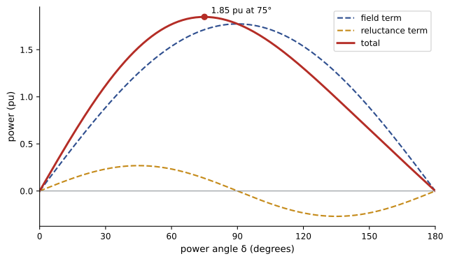
The reluctance term adds about 4% to the maximum power and moves the peak to about 75°, so the steady-state stability limit of a salient-pole machine is reached at a smaller angle than for a cylindrical rotor. With the field switched off, the machine can still carry 0.27 pu from reluctance alone, which is why a salient-pole synchronous motor that loses excitation may keep running at reduced load, and the principle behind synchronous reluctance motors (Lesson 11).

Sudden short circuit: subtransient and transient reactances

When a three-phase short circuit occurs at a generator's terminals, the armature current rises suddenly. The flux linking the rotor circuits cannot change instantly, so the rotor's field winding and damper (amortisseur) windings react by carrying induced currents that oppose the change, keeping the armature flux out of the rotor. The armature reaction flux is forced into high-reluctance leakage paths, so the effective reactance is small at first and grows as the induced rotor currents decay. Three periods are distinguished:

• Subtransient period (first few cycles): damper and field windings both oppose flux change; the reactance is the subtransient reactance \(X_d''\), typically 0.12 to 0.25 pu, and the current decays with time constant \(T_d''\) of about 0.02 to 0.05 s.
• Transient period (up to about a second or two): damper currents have decayed but the field winding still opposes the change; the reactance is the transient reactance \(X_d'\), typically 0.2 to 0.4 pu, decaying with \(T_d'\) of about 0.5 to 2 s.
• Steady state: the induced field current has decayed, and the current is limited by the synchronous reactance \(X_d\), typically 1.0 to 2.0 pu.

The symmetrical (AC) component of the short-circuit current is

In addition, each phase carries a DC offset that depends on the point on the voltage wave at which the fault occurs, decaying with the armature time constant \(T_a\). In the worst-case phase, the first peak is nearly twice the peak of the symmetrical current.

import numpy as np

# Symmetrical three-phase short circuit at the terminals of an unloaded generator (per unit, E = 1.0)
E = 1.0
Xd2, Xd1, Xd = 0.18, 0.30, 1.6           # subtransient, transient and synchronous reactances
Td2, Td1 = 0.035, 1.0                    # short-circuit subtransient and transient time constants (s)
Ta = 0.25                                 # armature (DC offset) time constant (s)

def ac_rms(t):
    return E / Xd + (E / Xd1 - E / Xd) * np.exp(-t / Td1) + (E / Xd2 - E / Xd1) * np.exp(-t / Td2)

for t_ms in (0, 50, 100, 300, 1000, 3000, 6000):
    t = t_ms / 1000
    print(f"t = {t_ms:5d} ms: symmetrical rms current {ac_rms(t):5.2f} pu")
peak = np.sqrt(2) * ac_rms(0) * (1 + np.exp(-0.5 / 60 / Ta))    # fully offset phase, first half-cycle peak
print(f"first peak in the fully offset phase about {peak:.1f} pu (instantaneous)")
I_base = 100e6 / (np.sqrt(3) * 13.8e3)
print(f"for a 100 MVA, 13.8 kV machine: initial {ac_rms(0) * I_base / 1000:.1f} kA rms, after 3 cycles {ac_rms(0.05) * I_base / 1000:.1f} kA, steady state {E / Xd * I_base / 1000:.1f} kA")

t =     0 ms: symmetrical rms current  5.56 pu
t =    50 ms: symmetrical rms current  3.73 pu
t =   100 ms: symmetrical rms current  3.20 pu
t =   300 ms: symmetrical rms current  2.63 pu
t =  1000 ms: symmetrical rms current  1.62 pu
t =  3000 ms: symmetrical rms current  0.76 pu
t =  6000 ms: symmetrical rms current  0.63 pu
first peak in the fully offset phase about 15.5 pu (instantaneous)
for a 100 MVA, 13.8 kV machine: initial 23.2 kA rms, after 3 cycles 15.6 kA, steady state 2.6 kA

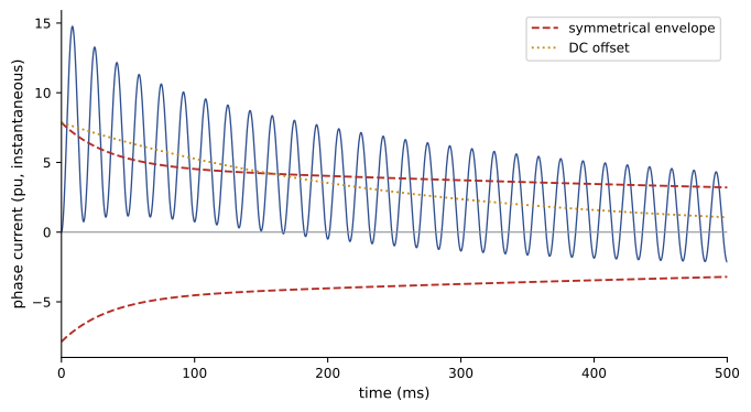
These values are used for different purposes. The subtransient current, about 5.6 pu here, with its DC offset, sets the momentary (first-cycle) duty of circuit breakers and the mechanical forces on bus bars and windings. The current a few cycles later, when breaker contacts part, sets the interrupting duty. The transient current governs the settings of time-delayed protection. The steady-state value, only 0.63 pu with constant excitation, is less than rated current: a generator with its excitation held constant cannot sustain a large fault current, which is why excitation systems provide field forcing and why generator backup protection uses voltage-restrained or voltage-controlled overcurrent relays (ELE-380 covers fault calculations).

The swing equation

In steady state, the generator's rotor turns at synchronous speed and the mechanical input power \(P_m\) from the turbine equals the electrical output \(P_e\). After a disturbance, the difference accelerates or decelerates the rotor, changing the rotor angle \(\delta\) relative to the synchronously rotating reference. With the inertia constant \(H\) defined as the stored kinetic energy at synchronous speed divided by the machine rating (in seconds), the swing equation in per unit is

where \(\omega_s = 2\pi f\) electrical rad/s. Typical values of \(H\) are 2 to 4 s for hydro units, 4 to 9 s for steam turbine generators, and much smaller for small machines. A large \(H\) means the rotor accelerates slowly, giving protection more time to clear a fault.

Transient stability and the equal-area criterion

Transient stability is the ability of a generator to remain in synchronism after a large disturbance such as a fault. During a fault near the generator, electrical output collapses while mechanical input continues, so the rotor accelerates and \(\delta\) increases. When the fault is cleared, electrical output exceeds mechanical input and the rotor decelerates; if it stops advancing before passing the point where electrical power falls back below mechanical power, the machine swings back and settles. Otherwise it slips a pole and loses synchronism.

For a single machine connected to a large system, the equal-area criterion decides stability without integrating the swing equation: the kinetic energy gained during acceleration, represented by the area between \(P_m\) and \(P_e\) during the fault, must be returned during deceleration, the area between the post-fault \(P_e\) curve and \(P_m\) before the angle reaches its limit \(\delta_{max} = \pi - \arcsin(P_m/P_{max})\). The angle at which the fault must be cleared for the two areas to be equal is the critical clearing angle, and the time to reach it is the critical clearing time.

import numpy as np

# Swing equation for a generator connected to an infinite bus through two parallel lines.
# A three-phase fault on one line near the bus drops electrical output to zero; the faulted line then trips.
H, f0 = 4.0, 60.0                      # inertia constant (s) and frequency
Pm = 0.9                               # mechanical input (pu)
E, V = 1.2, 1.0
X_pre, X_post = 0.55, 0.75             # transfer reactance before the fault and after the faulted line trips
Pmax_pre, Pmax_post = E * V / X_pre, E * V / X_post
d0 = np.arcsin(Pm / Pmax_pre)

def simulate(t_clear, t_end=2.0, dt=0.0005):
    d, w = d0, 0.0                     # rotor angle (rad) and speed deviation (rad/s)
    t, dmax = 0.0, d0
    while t < t_end:
        Pe = 0.0 if t < t_clear else Pmax_post * np.sin(d)
        w += np.pi * f0 / H * (Pm - Pe) * dt
        d += w * dt
        t += dt
        dmax = max(dmax, d)
        if d > np.pi:
            return False, dmax
    return True, dmax

print(f"initial angle {np.degrees(d0):.1f} deg; post-fault maximum power {Pmax_post:.2f} pu")
for cycles in (4, 6, 8, 10, 11, 12):
    ok, dmax = simulate(cycles / f0)
    status = f"stable, maximum angle {np.degrees(dmax):5.1f} deg" if ok else "unstable: loses synchronism (pole slip)"
    print(f"fault cleared in {cycles:2d} cycles ({cycles / f0 * 1000:4.0f} ms): {status}")
# Critical clearing angle from the equal-area criterion
dm = np.pi - np.arcsin(Pm / Pmax_post)
dc = np.arccos(Pm * (dm - d0) / Pmax_post + np.cos(dm))
tc = np.sqrt(2 * H * (dc - d0) / (np.pi * f0 * Pm))
print(f"equal-area criterion: critical clearing angle {np.degrees(dc):.1f} deg, critical clearing time {tc * 1000:.0f} ms ({tc * f0:.1f} cycles)")

initial angle 24.4 deg; post-fault maximum power 1.60 pu
fault cleared in  4 cycles (  67 ms): stable, maximum angle  56.5 deg
fault cleared in  6 cycles ( 100 ms): stable, maximum angle  67.9 deg
fault cleared in  8 cycles ( 133 ms): stable, maximum angle  83.4 deg
fault cleared in 10 cycles ( 167 ms): stable, maximum angle 105.9 deg
fault cleared in 11 cycles ( 183 ms): stable, maximum angle 124.2 deg
fault cleared in 12 cycles ( 200 ms): unstable: loses synchronism (pole slip)
equal-area criterion: critical clearing angle 68.6 deg, critical clearing time 191 ms (11.4 cycles)

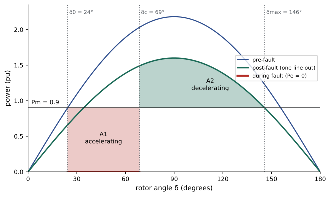
The simulation and the equal-area criterion agree: the generator survives faults cleared within 11 cycles (183 ms) and slips a pole at 12 cycles, matching the critical clearing time of about 191 ms. Modern protection clears transmission faults in 3 to 5 cycles, well within this margin, but a breaker failure that adds backup clearing time could exceed it. Ways to improve transient stability include faster protection and breakers, higher inertia, lower transfer reactance (more or stronger lines, series compensation), fast valving of steam turbines, braking resistors, and fast excitation systems with high ceiling voltage that raise \(E\) and hence \(P_{max}\) during the swing. Multi-machine stability studies, with detailed generator, exciter and governor models, are covered in ELE-380.

Excitation systems

The excitation system supplies DC field current and controls it with an automatic voltage regulator (AVR). Three main types are used:

• DC exciters: a DC generator on the shaft, now largely retired.
• Brushless AC exciters: a small inverted AC generator on the shaft, whose rotating armature output is rectified by diodes on the rotor and fed directly to the field; no brushes or slip rings, so maintenance is low. Response is moderate because the exciter field must change first.
• Static exciters: thyristor rectifiers fed from the generator terminals through a transformer, with slip rings to the field. They respond within a few cycles and have high ceiling voltages, giving the best transient stability support.

The AVR regulates terminal voltage and, together with limiters, keeps the machine within its capability curve (Lesson 9): over-excitation limiters protect the field from overheating, under-excitation limiters prevent loss of stability and stator end-core heating, and volts-per-hertz limiters prevent over-fluxing of the generator and its step-up transformer at low frequency.

Fast, high-gain AVRs improve transient stability but can reduce the damping of electromechanical oscillations, in which generators swing against each other at 0.2 to 2 Hz. A power system stabilizer (PSS) adds a supplementary signal, derived from shaft speed, frequency or electrical power, to the AVR so that the field produces torque in phase with speed deviations, damping the oscillations. Grid codes of Canadian and US system operators require PSS on large generators, and the 1996 western North American blackout highlighted the role of poorly damped inter-area oscillations.

Generator protection

Large generators are expensive and their failure can be catastrophic, so they have extensive protection, typically following IEEE C37.102:

• Stator differential protection (87G) for internal phase faults.
• Stator ground fault protection: generators are usually grounded through a high impedance (a distribution transformer with a resistor) to limit ground fault current to a few amperes; a neutral overvoltage relay and third-harmonic schemes together cover 100% of the winding.
• Loss of excitation (40), detected by impedance relays, because a generator that loses its field draws large reactive power from the system and overheats.
• Negative-sequence (46) protection against rotor heating from unbalanced faults and loads, which induce double-frequency rotor currents.
• Out-of-step (78) protection against pole slipping.
• Reverse power (32) protection against motoring, which can damage turbines.
• Over- and under-frequency (81), overexcitation (24), voltage-restrained overcurrent (51V), and field ground fault protection.