
ELE-351 · Lesson 8 of 12 · 23 min
FIR filter design
An FIR filter is a list of coefficients, and designing one means choosing that list so that the frequency response meets a specification with as few taps as possible. FIR filters are the workhorses of DSP for three reasons: they are always stable, they can have exactly linear phase, and their behavior in fixed-point arithmetic is benign and easy to predict. Their weakness is cost: a sharp FIR filter can need many more multiplies than an IIR filter with a similar magnitude response. CMP-450 implemented a 32-tap windowed-sinc FIR filter in an FPGA and studied its fixed-point behavior in detail. This lesson concentrates on design: the four types of linear-phase filter, the window method and the Kaiser formulas that size it, equiripple design by the Parks-McClellan algorithm, quick estimates of filter length, and the special half-band filters used in sample-rate conversion. The application is the interpolation filter that lets the APS-2 play its 16 kHz voice prompts through the 48 kHz DAC.
Writing the specification
A low-pass specification has four numbers: the pass-band edge f_p, the stop-band edge f_s (written f_stop here to avoid confusion with the sample rate), the allowed pass-band ripple δ_p and the required stop-band attenuation δ_s. Ripple in decibels is about 17.4δ_p for small δ_p, so ±0.1 dB is δ_p ≈ 0.0115. Stop-band attenuation A = −20 log₁₀ δ_s, so 70 dB is δ_s ≈ 0.000316. The difficulty of a design is set mostly by the transition width Δf = f_stop − f_p relative to the sample rate and by the attenuation; the required length is roughly proportional to A and inversely proportional to Δf/f_rate.
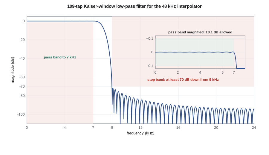
Amara's interpolation filter runs at 48 kHz on a signal that has been upsampled from 16 kHz by inserting two zeros after every sample, which lesson 11 explains. The upsampled signal contains the wanted spectrum from 0 to 8 kHz and two images, centered near 16 and 32 kHz, that the filter must remove. The voice prompts are recorded with content up to 7 kHz, so she sets f_p = 7 kHz with ±0.1 dB ripple. The first image of 7 kHz falls at 16 − 7 = 9 kHz, so f_stop = 9 kHz, with 70 dB of attenuation so that the images stay below the DAC's noise floor at normal listening levels. The transition band, 7 to 9 kHz, is only 2 kHz wide at a 48 kHz rate, a normalized width of 0.0417.
Linear-phase FIR filters
An FIR filter of length N has exactly linear phase if its coefficients are symmetric, h[n] = h[N − 1 − n], or antisymmetric, h[n] = −h[N − 1 − n]. Combined with N odd or even, that gives four types. Their difference lies in forced zeros. A symmetric filter of even length always has a zero at ω = π, so it cannot be a high-pass filter. Antisymmetric filters always have a zero at ω = 0, so they cannot pass DC, which suits differentiators and Hilbert transformers. The group delay of every type is (N − 1)/2 samples, which is a whole number of samples only for odd N. Symmetry also halves the multiplications, because pairs of samples sharing a coefficient can be added before multiplying; the pre-adder in CMP-450's FPGA design exploited exactly that.
| Type | Symmetry | Length N | Forced zeros | Suitable for |
|---|---|---|---|---|
| I | symmetric | odd | none | any response: low-pass, high-pass, bandpass, bandstop |
| II | symmetric | even | ω = π | low-pass and bandpass, not high-pass |
| III | antisymmetric | odd | ω = 0 and ω = π | Hilbert transformers, bandpass |
| IV | antisymmetric | even | ω = 0 | differentiators, Hilbert transformers, high-pass |
The window method
The ideal low-pass filter of lesson 5 has the impulse response sin(ω_c n)/(πn), infinite in both directions. The window method truncates it to N samples, shifts it to be causal, and multiplies it by a window to reduce the ripples that truncation causes. The cutoff ω_c is placed at the middle of the transition band. By the multiplication property, the resulting response is the ideal response convolved with the window's spectrum: the main-lobe width of the window sets the transition width, and its sidelobes set the ripple, which appears with nearly the same size in the pass band and the stop band. That last point is a limitation of the method: δ_p and δ_s come out about equal, so a filter designed to give 70 dB in the stop band has a pass band far flatter than ±0.1 dB, which wastes taps.
The fixed windows of lesson 6 give fixed attenuations. A rectangular window gives about 21 dB, Hann about 44 dB, Hamming about 53 dB and Blackman about 74 dB of stop-band attenuation, which are much better than the windows' own sidelobe levels because the convolution integrates the sidelobes. To reach a particular attenuation exactly, Kaiser's window adds a shape parameter β, and Kaiser gave empirical formulas for both β and the length. They are the quickest way to a good FIR filter.
The Kaiser window itself is built from the modified Bessel function I₀, which a short power series computes easily. Larger β gives a wider main lobe and lower sidelobes; β = 0 is the rectangular window, and β around 5 to 6 behaves much like Hamming.
Worked problem
Sizing the interpolation filter by Kaiser's formulas
Find β and the length for the APS-2 interpolation filter: f_p = 7 kHz, f_stop = 9 kHz at 48 kHz, 70 dB attenuation.
Show solution
- \[\Delta\omega = \frac{2\pi (9000 - 7000)}{48\,000} = 0.2618\ \text{rad/sample}\]
- \[\beta = 0.1102\,(70 - 8.7) = 6.755\]
- \[N - 1 \approx \frac{70 - 8}{2.285 \times 0.2618} = 103.6 \;\Rightarrow\; N = 105 \text{ (odd, type I)}\]
- \[\omega_c = \frac{2\pi\, (8000)}{48\,000} = \frac{\pi}{3}\]
Answer: The formulas call for about 105 taps, with the cutoff at 8 kHz, exactly f_rate/6, which makes every third coefficient after the center exactly zero, a property lesson 11 uses. Kaiser's formulas are empirical, so a design must always be measured; the code below builds the filter, finds it about half a decibel short, and raises the design attenuation until the measured stop band has a little margin.
Equiripple design
The window method spreads its error unevenly: the ripples are largest near the band edges and die away elsewhere, and the pass-band and stop-band errors are tied together. An optimal filter instead spreads the error evenly, with ripples of equal height across each band, and lets the designer weight the pass band and stop band separately. In 1972 Parks and McClellan published an algorithm, based on the Remez exchange method of approximation theory, that finds the filter of a given length that minimizes the largest weighted error. The result is equiripple: by the alternation theorem, the optimal error touches its maximum at least (N + 3)/2 times for an odd-length type I filter, alternating in sign. Every serious filter design package includes it, often called remez or firpm.
The algorithm itself is iterative and a little long to write from scratch, so in practice an engineer runs it in a design tool and pastes the coefficients into firmware. What matters for planning is how many taps it will need. A widely used estimate, also due to Kaiser, gives the length from both ripples; another, by Harris, gives a simpler rule of thumb. For Amara's specification, the two estimates give about 69 and 76 taps, roughly a third fewer than the Kaiser window design, because the pass band is allowed its full ±0.1 dB instead of the much smaller ripple the window method forces on it.
Other design methods
Two more methods are worth knowing. Frequency sampling specifies the desired response at N equally spaced frequencies, sets the coefficients by an inverse DFT, and optionally optimizes a few transition-band samples; it is simple and useful for filters with arbitrary shapes, such as a correction for a measured microphone response. Least-squares design minimizes the total squared error rather than the largest error; it gives lower average stop-band energy, which suits applications such as decimation where the total aliased noise matters more than the worst single frequency. Both are available in standard tools.
Half-band filters
A half-band filter is a type I low-pass filter whose transition band is centered exactly on a quarter of the sample rate, with equal pass-band and stop-band ripples. Its impulse response has a remarkable property: every other coefficient, apart from the center one, is exactly zero. A half-band filter of N taps therefore needs only about N/4 multiplies per output once symmetry is also used. That makes half-band filters the standard building block for changing rates by factors of two, and multistage decimators of lesson 11 chain several of them. Filters centered on f_rate/(2M) for other integers M, called Nyquist or M-th-band filters, have every M-th coefficient zero in the same way, which is why Amara's 8 kHz cutoff at a 48 kHz rate gives zeros at every third coefficient.
import math, cmath
def i0(x):
    s, t, k = 1.0, 1.0, 1
    while t > 1e-12 * s:
        t *= (x / (2 * k)) ** 2; s += t; k += 1
    return s
def kaiser_lowpass(fp, fst, A, fr):
    dw = 2 * math.pi * (fst - fp) / fr
    beta = 0.1102 * (A - 8.7) if A > 50 else (0.5842 * (A - 21) ** 0.4 + 0.07886 * (A - 21) if A >= 21 else 0.0)
    N = math.ceil((A - 8) / (2.285 * dw)) + 1
    if N % 2 == 0: N += 1
    wc = math.pi * (fp + fst) / fr; a = (N - 1) / 2
    h = []
    for n in range(N):
        m = n - a
        ideal = wc / math.pi if m == 0 else math.sin(wc * m) / (math.pi * m)
        h.append(ideal * i0(beta * math.sqrt(1 - (2 * n / (N - 1) - 1) ** 2)) / i0(beta))
    return h, beta
def mag_db(h, f, fr):
    z = cmath.exp(-2j * math.pi * f / fr)
    return 20 * math.log10(abs(sum(c * z ** n for n, c in enumerate(h))))
fr = 48000
A_design = 70.0
while True:
    h, beta = kaiser_lowpass(7000, 9000, A_design, fr)
    pb = [mag_db(h, f, fr) for f in range(0, 7001, 50)]
    sb = [mag_db(h, f, fr) for f in range(9000, 24001, 50)]
    print(f"design A = {A_design:.1f} dB: beta = {beta:.3f}, N = {len(h)} taps, pass band {min(pb):+.4f} to {max(pb):+.4f} dB, stop band worst {max(sb):.1f} dB")
    if max(sb) <= -70.5: break       # keep 0.5 dB of margin
    A_design += 1.0
print(f"accepted N = {len(h)}, group delay {(len(h)-1)//2} samples = {1000*(len(h)-1)/2/fr:.2f} ms")
print("symmetric:", all(abs(h[n] - h[len(h) - 1 - n]) < 1e-15 for n in range(len(h))))
c = (len(h) - 1) // 2
print("coefficients at middle + 3k (k = 1..4):", [f"{h[c + 3*k]:.1e}" for k in range(1, 5)])
dp = 10 ** (0.1 / 20) - 1; ds = 10 ** (-70 / 20)
for name, fn in (("Kaiser equiripple estimate", lambda: (-20 * math.log10(math.sqrt(dp * ds)) - 13) / (14.6 * 2000 / fr) + 1),
                 ("Harris rule of thumb", lambda: 70 / (22 * 2000 / fr))):
    print(f"{name}: about {fn():.0f} taps")
symm_mults = (len(h) + 1) // 2
nonzero = sum(1 for v in h if abs(v) > 1e-12)
print(f"multiplies per output at 48 kHz: direct {len(h)}, using symmetry {symm_mults}, nonzero coefficients {nonzero}")design A = 70.0 dB: beta = 6.755, N = 105 taps, pass band -0.0024 to +0.0030 dB, stop band worst -69.6 dB design A = 71.0 dB: beta = 6.865, N = 107 taps, pass band -0.0019 to +0.0027 dB, stop band worst -70.0 dB design A = 72.0 dB: beta = 6.976, N = 109 taps, pass band -0.0016 to +0.0021 dB, stop band worst -72.1 dB accepted N = 109, group delay 54 samples = 1.12 ms symmetric: True coefficients at middle + 3k (k = 1..4): ['1.3e-17', '-1.2e-17', '1.2e-17', '-1.1e-17'] Kaiser equiripple estimate: about 69 taps Harris rule of thumb: about 76 taps multiplies per output at 48 kHz: direct 109, using symmetry 55, nonzero coefficients 73
The first Kaiser design, at the formula's 105 taps, reaches only −69.6 dB. Designing for 72 dB gives 109 taps and a measured −72.1 dB, which meets the specification with margin. Its pass band is flat to within a few thousandths of a decibel, far better than the ±0.1 dB allowed, which is the window method's typical waste. The coefficients at three, six, nine and twelve taps from the center are zero to machine precision, as predicted for a cutoff at f_rate/6. The equiripple estimates of about 70 to 76 taps show what an optimal design would save. Amara decides to use the Kaiser design in the first firmware, because it can be computed on the device from four parameters, and to replace it with an equiripple design from the team's design tool once the specification is frozen. Either way, lesson 11 shows that the polyphase implementation never multiplies by the inserted zeros, so the real cost is about a third of these counts.
Checking a design before it ships
A filter design is not finished when the plot looks good. Amara's review checklist asks for four checks. The response must meet the specification on a dense frequency grid, including the band edges, not just at a few points. The coefficients must be checked after quantization to the firmware's word length, because rounding raises the stop-band floor; CMP-450's lesson on bit-accurate FIR models showed how 16-bit coefficients can limit a 70 dB design and how many accumulator bits are needed. The impulse and step responses must be inspected for excessive ringing, which in audio can be heard as pre-echo in front of sharp sounds because a linear-phase filter rings before its main peak as well as after. And the filter must be tested in the firmware with a swept tone and with white noise, comparing the measured response with the design.
Common mistakes
MistakeChoosing an even length for a high-pass linear-phase FIR filter.
InsteadType II filters have a forced zero at the Nyquist frequency; use an odd length (type I).
MistakePlacing the window-method cutoff at the pass-band edge.
InsteadPut ω_c in the middle of the transition band; the window spreads the edge symmetrically.
MistakeExpecting the window method to give independent pass-band and stop-band ripple.
InsteadWindow designs have δ_p ≈ δ_s; use equiripple design with weights to set them separately.
MistakeIgnoring coefficient quantization.
InsteadRounding coefficients to 16 bits can raise the stop band above −80 to −90 dB; check the quantized response.
Summary and key terms
- A specification gives pass-band and stop-band edges and ripples; length grows with attenuation and falls with transition width.
- Symmetric or antisymmetric coefficients give exactly linear phase; the four types differ in forced zeros at ω = 0 and π.
- The window method truncates and windows the ideal impulse response; Kaiser's formulas give β and length from A and Δω.
- Parks-McClellan equiripple design minimizes the largest weighted error and usually needs fewer taps than a window design.
- Length estimates by Kaiser and Harris let an engineer budget cycles before designing.
- Half-band and M-th-band filters have regularly spaced zero coefficients and are efficient for rate conversion.
- Pass-band ripple
- The allowed deviation of the gain from its nominal value in the pass band.
- Stop-band attenuation
- The minimum loss required in the stop band, usually in decibels.
- Transition band
- The band between pass-band and stop-band edges.
- Window method
- FIR design by multiplying the ideal impulse response by a finite window.
- Kaiser window
- A window with a shape parameter β that trades main-lobe width against sidelobe level.
- Equiripple filter
- A filter whose error ripples have equal peak height across each band.
- Parks-McClellan algorithm
- An iterative algorithm that finds the optimal equiripple linear-phase FIR filter.
- Half-band filter
- A low-pass FIR filter with cutoff at a quarter of the sample rate in which every other coefficient is zero.
Practice problems
Work each problem on paper first, then reveal the answer to check.
Convert ±0.05 dB ripple and 60 dB attenuation to δ_p and δ_s.
Show answer
δ_p ≈ 10^(0.05/20) − 1 = 0.0058; δ_s = 10⁻³.
Using Kaiser's formula, find β and N for A = 50 dB and Δω = 0.1π.
Show answer
β = 0.5842(29)^0.4 + 0.07886(29) = 4.53; N − 1 = 42/(2.285 × 0.314) = 58.5, so N = 60 (or 61 for type I).
A type II FIR filter is proposed as a high-pass filter. What is wrong?
Show answer
It has a forced zero at ω = π, exactly where a high-pass filter must pass.
What is the group delay of a 75-tap linear-phase filter at 48 kHz?
Show answer
37 samples = 0.77 ms.
With the Harris rule, estimate the taps for 80 dB with a transition of 1 kHz at 16 kHz.
Show answer
80/(22 × 1/16) = 58 taps.
How many multiplies per output does a 63-tap half-band filter need when symmetry and zero coefficients are both used?
Show answer
About 16 distinct nonzero coefficient pairs plus the center, roughly 17.
Lesson quiz · 5 questions
Score 60% or more to complete this lesson.
Create a free account to save your progress, take quizzes and earn a certificate.