
ELE-351 · Lesson 7 of 12 · 20 min
The fast Fourier transform
Computed straight from its definition, an N-point DFT needs N² complex multiplications: for every one of N outputs, a sum of N products. For N = 1024 that is over a million multiplications per transform, too many for a small processor to do often. The fast Fourier transform (FFT) computes exactly the same result with about (N/2) log₂ N multiplications, roughly 5000 for N = 1024, by reusing intermediate results. The FFT, published in its modern form by Cooley and Tukey in the 1960s, is one of the most important algorithms in engineering. ELE-250 showed a short recursive FFT. This lesson looks inside it: the decimation-in-time derivation, butterflies and bit reversal, in-place computation, operation counts, real-input tricks, fixed-point scaling, and the most important use of the FFT after spectrum analysis, fast convolution of long signals.
Divide and conquer
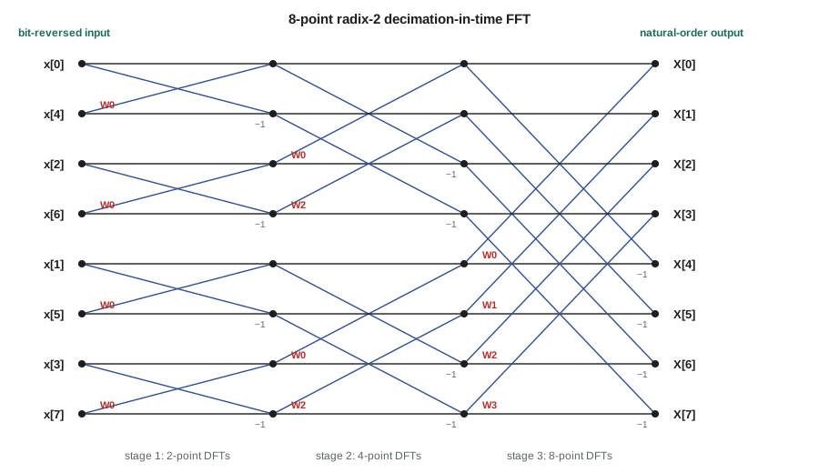
The radix-2 decimation-in-time FFT splits an N-point DFT, with N a power of two, into two N/2-point DFTs, one of the even-indexed samples and one of the odd-indexed samples. Because the twiddle factor W_N = e^(−j2π/N) has the property W_N² = W_(N/2), each half is itself a DFT of half the length. The two halves, E[k] and O[k], combine to give the full transform in two lines, one for the first half of the outputs and one for the second, sharing the same product W_N^k O[k].
This pair of equations is the butterfly: two inputs, one complex multiplication by a twiddle factor, one addition and one subtraction, two outputs. Applying the split recursively until the transforms have length 1, which is just the sample itself, gives log₂ N stages of N/2 butterflies each. The total is (N/2) log₂ N complex multiplications and N log₂ N complex additions. Some of the multiplications are by 1 or −j and cost nothing, so practical counts are a little lower.
Bit reversal and in-place computation
Following the even-odd splits all the way down puts the input samples in a scrambled order. Sample n ends up at the position given by writing n in binary with log₂ N bits and reversing the bits: for N = 8, sample 1 (001) goes to position 4 (100), and sample 3 (011) to position 6 (110). An iterative FFT therefore starts by reordering the input into bit-reversed order, then runs the stages. Each butterfly reads two values and writes two values back to the same two memory locations, so the whole transform can be done in place, needing no extra memory beyond the twiddle-factor table. That is why FFT libraries for microcontrollers often require power-of-two lengths and operate on a single array.
The decimation-in-frequency FFT is the mirror image: it splits the outputs rather than the inputs into even and odd halves, so its inputs are in natural order and its outputs come out bit-reversed. The two forms have the same cost. Faster variants exist. Radix-4 algorithms combine two stages into one and save about 25 percent of the multiplications; split-radix saves a little more. Lengths that are not powers of two, such as 600 or 400, are handled by mixed-radix algorithms that factor N into small primes, and arbitrary lengths, including primes, by algorithms that turn a DFT into a convolution. For the APS-2, Amara uses the processor vendor's optimized radix-4 library for 256 points, and keeps a mixed-radix path for the 400-point locator-tone check of lesson 6.
How much faster?
| N | Direct DFT, complex multiplies | Radix-2 FFT, complex multiplies | Speed-up |
|---|---|---|---|
| 64 | 4 096 | 192 | 21 |
| 256 | 65 536 | 1 024 | 64 |
| 1 024 | 1 048 576 | 5 120 | 205 |
| 4 096 | 16 777 216 | 24 576 | 683 |
| 65 536 | 4.3 × 10⁹ | 524 288 | 8 192 |
The speed-up grows with N, roughly as 2N/log₂ N. For the APS-2 spectrum monitor, one 256-point FFT takes about a thousand complex multiplies, each of which is four real multiplies and two additions; on a processor with a single-cycle MAC, an optimized 256-point complex FFT runs in a few thousand cycles. A hundred of them per second, for a Welch estimate updated once a second, uses well under one percent of the processor.
Real-valued inputs
Audio samples are real, but the FFT is a complex algorithm. Feeding it real data with zero imaginary parts wastes half its work. Two standard tricks recover the waste. The first transforms two real sequences at once: put one in the real part and one in the imaginary part, take one complex FFT, then separate the two spectra using conjugate symmetry. The second transforms one real sequence of length N with a complex FFT of length N/2: pack even samples into the real part and odd samples into the imaginary part, transform, and apply one extra pass of butterflies to untangle the result. Either way, a real FFT costs about half of a complex one of the same length.
The inverse DFT needs no separate algorithm either. Conjugating the input, applying the forward FFT, conjugating the output and dividing by N gives the inverse transform. Most libraries provide both directions, but the trick is handy in a pinch, and it shows that the two transforms have exactly the same cost.
Fixed-point FFTs
In fixed-point arithmetic, the FFT's additions can overflow. A butterfly can double the magnitude of its outputs, so after log₂ N stages the values can grow by a factor of N, which is 8 bits for N = 256. There are three standard remedies. Scaling each stage by 1/2 guarantees no overflow but costs precision: each halving discards a bit and adds rounding noise, and the output is the DFT divided by N. Scaling the input down by N at the start avoids rounding inside but throws away low-level detail. Block floating point checks the largest value after each stage and scales only when needed, keeping a shared exponent; it gives nearly floating-point quality and is what many DSP libraries do. For a 16-bit FFT with per-stage scaling, the output SNR for a full-scale input is roughly 6 dB worse for every factor of four in N, which is why the APS-2 spectrum monitor runs its FFT in 32-bit fixed point or single-precision floating point.
Fast convolution
Lesson 6 showed that multiplying zero-padded DFTs gives linear convolution. With the FFT, that becomes faster than direct convolution for long filters. A filter of M taps applied directly costs M multiplies per output sample. Applied by FFT, the input is cut into blocks of L samples, each block is zero-padded to N ≥ L + M − 1, transformed, multiplied by the precomputed transform of the filter, and transformed back. The blocks' outputs are each L + M − 1 long and overlap their neighbors by M − 1 samples, so they are added together: this is the overlap-add method. Overlap-save is equivalent: it overlaps the input blocks instead, and discards the M − 1 wrapped samples at the start of each output block.
The crossover point depends on the processor and the library, but as a rough guide, fast convolution starts to win somewhere between 32 and 128 taps and wins decisively for hundreds or thousands. The price is latency: a block of L samples must arrive before any of its output can be computed. Echo cancellers in teleconferencing systems with filters of thousands of taps use partitioned frequency-domain methods to keep the cost down and the latency short. The APS-2 echo path is short, a few milliseconds from speaker to microphone through the pole housing, so its echo canceller of lesson 12 runs directly in the time domain.
Worked problem
Choosing a convolution method
Leo needs to apply a measured 512-tap acoustic response to a 16 kHz test signal in the production test station. Compare direct convolution with overlap-add using 1024-point FFTs.
Show solution
- Direct convolution: 512 real multiplies per output sample.
- \[L = N - M + 1 = 1024 - 512 + 1 = 513 \text{ new outputs per block}\]
- \[\text{FFT cost} \approx 2 \times \Big(\frac{1024}{2}\times 10\Big) \times 4 + 4\times 1024 = 45\,056 \text{ real multiplies per block}\]
- \[\frac{45\,056}{513} \approx 88 \text{ real multiplies per output sample}\]
Answer: Overlap-add needs about 88 multiplies per output against 512 for direct convolution, nearly six times fewer, and the code below shows that the results are identical to within rounding. A longer FFT, 2048 points, would bring the cost down further, at the price of more memory and a longer block delay.
import cmath, math, random
def fft(a, inverse=False):                 # iterative in-place radix-2 FFT
    a = list(a); N = len(a); bits = N.bit_length() - 1
    for i in range(N):                     # bit-reversal permutation
        j = int(format(i, f'0{bits}b')[::-1], 2)
        if j > i: a[i], a[j] = a[j], a[i]
    size = 2
    while size <= N:
        w = cmath.exp((2j if inverse else -2j) * math.pi / size)
        for start in range(0, N, size):
            wk = 1
            for k in range(size // 2):
                u, t = a[start + k], wk * a[start + k + size // 2]
                a[start + k], a[start + k + size // 2] = u + t, u - t
                wk *= w
        size *= 2
    return [v / N for v in a] if inverse else a
random.seed(1)
x = [complex(random.uniform(-1, 1), 0) for _ in range(64)]
direct = [sum(x[n] * cmath.exp(-2j * math.pi * k * n / 64) for n in range(64)) for k in range(64)]
print("max |FFT - direct DFT| for N = 64:", f"{max(abs(p - q) for p, q in zip(fft(x), direct)):.2e}")
print("bit reversal for N = 8:", [int(format(i, '03b')[::-1], 2) for i in range(8)])
for N in (64, 256, 1024, 4096):
    print(f"N = {N:5d}: direct {N*N:9d}, FFT {N//2*int(math.log2(N)):7d}, speed-up {N*N/(N//2*math.log2(N)):6.0f}")
# real-input trick: two real sequences in one complex FFT
u = [random.uniform(-1, 1) for _ in range(16)]; v = [random.uniform(-1, 1) for _ in range(16)]
Z = fft([complex(p, q) for p, q in zip(u, v)])
U = [(Z[k] + Z[-k % 16].conjugate()) / 2 for k in range(16)]
print("two-for-one real FFT error:", f"{max(abs(p - q) for p, q in zip(U, fft(u))):.2e}")
# overlap-add with a 512-tap filter, 1024-point FFTs
M, N = 512, 1024; L = N - M + 1
h = [random.gauss(0, 1) * math.exp(-n / 80) for n in range(M)]
sig = [random.uniform(-1, 1) for _ in range(3 * L)]
H = fft(h + [0] * (N - M)); y = [0.0] * (len(sig) + M - 1)
for s0 in range(0, len(sig), L):
    blk = sig[s0:s0 + L]
    Y = fft([X * Hk for X, Hk in zip(fft(blk + [0] * (N - len(blk))), H)], inverse=True)
    for i in range(min(N, len(y) - s0)): y[s0 + i] += Y[i].real
check = [sum(h[k] * sig[n - k] for k in range(M) if 0 <= n - k < len(sig)) for n in range(0, len(y), 97)]
print("overlap-add vs direct, max error:", f"{max(abs(y[n] - c) for n, c in zip(range(0, len(y), 97), check)):.2e}")
fft_cost = 2 * (N // 2 * int(math.log2(N))) * 4 + 4 * N
print(f"real multiplies per output: direct {M}, overlap-add {fft_cost / L:.0f}")max |FFT - direct DFT| for N = 64: 1.53e-13 bit reversal for N = 8: [0, 4, 2, 6, 1, 5, 3, 7] N = 64: direct 4096, FFT 192, speed-up 21 N = 256: direct 65536, FFT 1024, speed-up 64 N = 1024: direct 1048576, FFT 5120, speed-up 205 N = 4096: direct 16777216, FFT 24576, speed-up 683 two-for-one real FFT error: 8.01e-16 overlap-add vs direct, max error: 1.08e-13 real multiplies per output: direct 512, overlap-add 88
The iterative FFT agrees with the direct DFT to about 10⁻¹³, close to the limit of double-precision arithmetic, and the bit-reversal table for N = 8 matches the figure. The two-for-one trick recovers the spectrum of one real sequence exactly from a shared complex transform. Overlap-add agrees with direct convolution to rounding error, and the cost comparison confirms the worked example.
FFT pitfalls
A few traps catch engineers who use FFT libraries without reading the documentation. Libraries differ in scaling: some scale the forward transform by 1/N, some the inverse, some neither, and some by 1/√N both ways. Output ordering differs: some return bins 0 to N − 1, some reorder to put DC in the middle, and in-place routines may leave the output bit-reversed. Real-input routines often return only N/2 + 1 bins, with the DC and Nyquist bins packed together. And a fixed-point routine that scales per stage returns the DFT divided by N, which must be undone when calibrating levels. Amara's rule for the team is simple: before trusting any FFT routine, feed it a known tone on a bin and a known white noise, and check that the tone amplitude and the noise PSD come out exactly as lessons 3 and 6 predict.
Common mistakes
MistakeComputing a few bins with a full FFT when only one or two frequencies are needed.
InsteadFor K bins with K small compared with log₂ N, direct evaluation or the Goertzel algorithm of lesson 12 is cheaper.
MistakeForgetting the bit-reversed order in an in-place FFT.
InsteadEither reorder the input first or read the output in bit-reversed order, depending on the algorithm.
MistakeRunning a 16-bit fixed-point FFT without scaling.
InsteadValues can grow by N; scale each stage, scale the input or use block floating point.
MistakeUsing overlap-add for every filter.
InsteadFor short filters, direct convolution is cheaper and has less latency; fast convolution pays off for long filters.
Summary and key terms
- The FFT computes the DFT exactly in about (N/2) log₂ N complex multiplications instead of N².
- Radix-2 decimation in time splits the input into even and odd halves; butterflies combine them with twiddle factors.
- In-place FFTs use bit-reversed ordering at the input or output and need no extra memory.
- Real-input data can be transformed at about half the complex cost by packing two sequences or the even and odd samples.
- Fixed-point FFTs need stage scaling or block floating point to avoid overflow, at some cost in precision.
- Overlap-add and overlap-save convolve long signals with long filters much faster than direct convolution, with a block of added latency.
- FFT
- Any fast algorithm that computes the DFT exactly with far fewer operations than the direct sum.
- Twiddle factor
- A complex exponential W_N^k = e^(−j2πk/N) that multiplies one input of a butterfly.
- Butterfly
- The basic FFT computation that combines two values with one twiddle multiplication, an addition and a subtraction.
- Bit reversal
- Reordering samples by reversing the binary digits of their index.
- In-place computation
- An algorithm that overwrites its input array with its results.
- Block floating point
- A fixed-point method that scales a whole array by a shared exponent only when needed.
- Overlap-add
- Fast convolution by adding the overlapping outputs of FFT-filtered input blocks.
- Overlap-save
- Fast convolution by overlapping input blocks and discarding wrapped output samples.
Practice problems
Work each problem on paper first, then reveal the answer to check.
How many butterflies does a 512-point radix-2 FFT contain?
Show answer
(512/2) × 9 = 2304.
Where does sample 6 go in bit-reversed order for N = 16?
Show answer
6 = 0110 → 0110 reversed is 0110 = 6; it stays in place.
Estimate the speed-up of a 2048-point FFT over a direct DFT.
Show answer
2048²/(1024 × 11) ≈ 372.
How many bits of growth must a fixed-point 1024-point FFT allow without scaling?
Show answer
log₂ 1024 = 10 bits.
A 200-tap filter is applied by overlap-add with 512-point FFTs. How many new outputs does each block give?
Show answer
512 − 200 + 1 = 313.
How can a forward FFT routine compute an inverse DFT?
Show answer
Conjugate the input, apply the forward FFT, conjugate the output and divide by N.
Lesson quiz · 5 questions
Score 60% or more to complete this lesson.
Create a free account to save your progress, take quizzes and earn a certificate.