
ELE-351 · Lesson 1 of 12 · 23 min
Discrete-time signals and systems
Digital signal processing, usually shortened to DSP, is the art of doing to a stream of numbers what analog circuits do to a voltage: filtering it, measuring it, mixing it, detecting things in it and shaping it for output. The numbers come from an analog-to-digital converter that samples a sensor, and they leave through a digital-to-analog converter or as decisions and data. In between, a processor runs arithmetic that never drifts with temperature, never ages and can be changed with a firmware update. This course takes the signals and systems theory of ELE-250 and turns it into working engineering: how to sample and quantize without losing what matters, how to compute spectra quickly and correctly, how to design FIR and IIR filters to a specification, how to implement them in finite-precision arithmetic, how to change sample rates efficiently and how to build filters that adapt themselves.
The course follows one product. At Cedarline Controls in Madison, the APS-2 accessible pedestrian signal push-button station is moving to revision C. Earlier courses designed its microphone receiver and speaker amplifier (ELE-340) and the TLR-1 telemetry radio that links it to the controller cabinet (ELE-350). Revision C replaces the old 8 kHz audio path and its analog filters with a modern audio codec and a 150 MHz microcontroller with DSP instructions. Daniel Fortin, PE, has asked Amara Osei to own the signal processing firmware, and Leo Tremblay, the co-op student, will build the test signals and run the measurements.
An accessible pedestrian signal speaks to people who are blind or have low vision. It plays a quiet locator tone so a person can find the push button, announces the street name and plays a walk indication when the walk interval starts. The hard part is volume. The sound must be heard at the crosswalk on a noisy afternoon, yet not annoy residents at night or be mistaken for the signal on another crossing. The APS-2 therefore listens to the street through its own microphone, estimates the ambient sound level and sets its output a few decibels above it. Every part of that job is signal processing, and each lesson of the course will add a piece of the revision C firmware.
The revision C signal chain
Amara starts by drawing the chain. The microphone feeds the differential receiver and preamplifier from ELE-340, then a stereo audio codec whose sigma-delta converter samples at 48 kHz with 24-bit words. The microcontroller first removes the 60 Hz hum and wind rumble with a high-pass filter, then decimates the stream by 3 to 16 kHz, because nothing above 8 kHz matters for level measurement. At 16 kHz it applies an A-weighting filter, which mimics the ear's sensitivity, and measures the ambient level. An echo canceller removes the APS-2's own sound from the microphone signal, so the device does not chase its own output upward. On the output side, stored voice messages recorded at 16 kHz are interpolated to 48 kHz, mixed with the locator tone and scaled by the volume control before they reach the DAC and the 4 W amplifier.
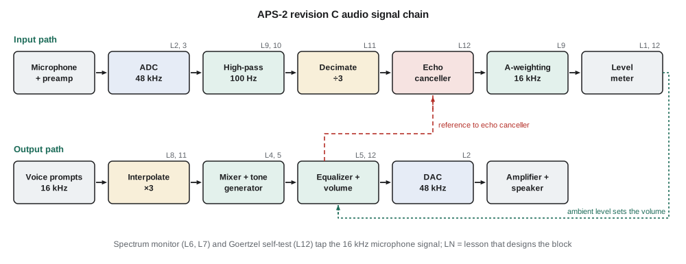
| Block | Sample rate | Purpose | Lesson |
|---|---|---|---|
| Sigma-delta ADC and DAC | 48 kHz | Convert between analog and digital audio | 2, 3 |
| High-pass filter | 48 kHz | Remove 60 Hz hum and wind rumble below about 100 Hz | 9, 10 |
| Decimator by 3 | 48 to 16 kHz | Reduce the rate for analysis | 11 |
| Echo canceller | 16 kHz | Remove the device's own sound from the microphone signal | 12 |
| A-weighting and level meter | 16 kHz | Estimate ambient sound level as the ear perceives it | 9, 12 |
| Spectrum monitor | 16 kHz | Diagnose noise sources and verify tones with the FFT | 6, 7 |
| Interpolator by 3 | 16 to 48 kHz | Play voice messages through the 48 kHz DAC | 8, 11 |
| Tone generator and mixer | 48 kHz | Make the locator and walk tones | 4, 5 |
Discrete-time signals
A discrete-time signal is a sequence of numbers x[n], indexed by an integer n. When it comes from sampling a continuous signal x(t) every T seconds, x[n] = x(nT), and the sample rate is f_s = 1/T. Square brackets mark the integer index; round brackets mark continuous time. A handful of sequences are used constantly. The unit impulse δ[n] is 1 at n = 0 and 0 elsewhere. The unit step u[n] is 1 for n ≥ 0 and 0 for n < 0. A real exponential aⁿu[n] decays when |a| < 1. A sinusoid A cos(ω₀n + φ) has a frequency ω₀ in radians per sample.
That last unit deserves attention, because it is where students of DSP most often go wrong. A continuous sinusoid of frequency f hertz, sampled at f_s, becomes a sequence with normalized frequency ω₀ = 2πf/f_s radians per sample. The 880 Hz locator tone sampled at 48 kHz has ω₀ = 2π × 880/48 000 = 0.1152 rad/sample, and the same tone sampled at 16 kHz has ω₀ = 0.3456 rad/sample. The frequency of a discrete sinusoid is only defined modulo 2π, because cos((ω₀ + 2π)n) = cos(ω₀n) for every integer n. All the distinct frequencies therefore live in the range −π to π, which corresponds to −f_s/2 to f_s/2. Anything outside that range is an alias of something inside it, which lesson 2 develops.
A discrete sinusoid is periodic only if ω₀/2π is a ratio of integers. The 880 Hz tone at 48 kHz has ω₀/2π = 880/48 000 = 11/600, so the sample pattern repeats exactly every 600 samples, which is 12.5 ms, containing 11 cycles of the tone. That fact is useful later: a table of 600 samples can generate the tone without any trigonometry at run time, and a DFT of 600 samples puts the tone exactly on a bin.
Systems and difference equations
A discrete-time system maps an input sequence to an output sequence. Almost every useful DSP system is described by a linear constant-coefficient difference equation, in which each output sample is a weighted sum of present and past inputs and past outputs. The coefficients b_k act on the input and a_k on past outputs. If all a_k are zero, the output depends only on a finite number of inputs, and the impulse response has finite length; this is a finite impulse response (FIR) system. If any a_k is nonzero, the output feeds back, and the impulse response usually lasts forever; this is an infinite impulse response (IIR) system.
ELE-250 defined the properties that matter: linearity, time invariance, causality and bounded-input bounded-output stability. A system described by a difference equation with fixed coefficients and zero initial conditions is linear and time invariant (LTI), so it is completely described by its impulse response h[n], the output when the input is δ[n]. A causal system has h[n] = 0 for n < 0, and it is stable if the sum of |h[n]| is finite. Every FIR filter is stable. An IIR filter is stable only if its feedback dies away, which lesson 4 relates to the positions of its poles.
Convolution
For an LTI system, the output is the convolution of the input with the impulse response. Each input sample launches a scaled, delayed copy of h[n], and the output is the sum of all those copies. In an FIR filter with M + 1 taps, convolution is exactly the difference equation: multiply the last M + 1 inputs by the coefficients and add. The operation count is one multiply and one add per tap per output sample, a multiply-accumulate or MAC, which is why DSP processors and microcontrollers with DSP extensions are built around a fast MAC instruction.
Worked problem
Convolution by hand
Leo feeds the sequence x[n] = 1, 2, 3 (for n = 0, 1, 2) into the three-tap smoother h[n] = 0.25, 0.5, 0.25. Find the output.
Show solution
- The output length is 3 + 3 − 1 = 5 samples.
- \[y[0] = 0.25(1) = 0.25 \qquad y[1] = 0.25(2) + 0.5(1) = 1.0\]
- \[y[2] = 0.25(3) + 0.5(2) + 0.25(1) = 2.0 \qquad y[3] = 0.5(3) + 0.25(2) = 2.0\]
- \[y[4] = 0.25(3) = 0.75\]
Answer: The output is 0.25, 1.0, 2.0, 2.0, 0.75. The coefficients sum to 1, so the area of the input (6) is preserved in the output (6.0), and the sharp edges of the input have been rounded off.
Two simple averagers
The level meter of the APS-2 needs an average of the squared microphone signal. Two averagers appear again and again in DSP firmware. The moving average of length L is an FIR filter whose L coefficients all equal 1/L. It forgets old samples completely after L samples, and it can be computed with one add and one subtract per sample by keeping a running sum. The exponential averager is the simplest IIR filter, y[n] = y[n − 1] + α(x[n] − y[n − 1]), with 0 < α < 1. It needs one multiply, keeps only one number of state and weights past inputs by a geometric series that never quite ends.
The time constant of the exponential averager follows from comparing its step response, 1 − (1 − α)^(n+1), with the analog 1 − e^(−t/τ). For small α, (1 − α)ⁿ ≈ e^(−αn), so the time constant is about T/α seconds. Sound level meters use standard time weightings: fast is 125 ms and slow is 1 s. At 16 kHz, a fast time weighting needs α ≈ 1/(0.125 × 16 000) = 0.0005, and a slow one α ≈ 0.0000625. Numbers that small are a hint of the word-length trouble lesson 10 will deal with: in 16-bit arithmetic, α × x can round to zero for small inputs and the averager stalls.
Real-time processing and the cycle budget
A DSP program must keep up with the converter. At 48 kHz a new sample arrives every 20.8 µs, and the processor must finish all the work for that sample, or for a block of samples, before the next one is due. A 150 MHz processor has 150 × 10⁶/48 000 = 3125 clock cycles per sample at 48 kHz. Amara's first engineering document is a cycle budget that lists every block, its rate and its cost, and checks that the total leaves a healthy margin for interrupts, the TLR-1 radio stack and future features.
Most firmware processes blocks rather than single samples. The codec fills a buffer of, say, 48 samples by direct memory access while the processor works on the previous 48; this double buffering, also called ping-pong buffering, cuts interrupt overhead and lets loops run efficiently. The price is latency: a 48-sample block adds at least 1 ms of input delay and 1 ms of output delay. For an APS that is harmless, but for the echo canceller of lesson 12 the delay must be known exactly, because the canceller has to line up the reference signal with its echo. A circular buffer, indexed modulo its length, holds the past inputs an FIR filter needs without moving data in memory.
# Cycle budget, convolution check and averager time constant for the APS-2 revision C firmware
f_cpu = 150e6
blocks = [  # name, sample rate (Hz), cycles per sample (estimates)
    ("high-pass biquads", 48000, 40),
    ("decimate by 3 (polyphase FIR)", 48000, 30),
    ("echo canceller (NLMS, 128 taps)", 16000, 520),
    ("A-weighting (3 biquads)", 16000, 60),
    ("level meter", 16000, 10),
    ("interpolate by 3 (polyphase FIR)", 48000, 30),
    ("tone, mix and volume", 48000, 25),
]
total = 0.0
for name, fs, cyc in blocks:
    load = fs * cyc / f_cpu
    total += load
    print(f"{name:34s} {100*load:5.2f} % of the processor")
print(f"{'total':34s} {100*total:5.2f} %   (cycles per 48 kHz sample available: {f_cpu/48000:.0f})")

def conv(x, h):
    y = [0.0] * (len(x) + len(h) - 1)
    for i, xv in enumerate(x):
        for k, hv in enumerate(h):
            y[i + k] += xv * hv
    return y
print("convolution:", conv([1, 2, 3], [0.25, 0.5, 0.25]))

fs = 16000
for name, tau in (("fast", 0.125), ("slow", 1.0)):
    alpha = 1 / (tau * fs)
    y, n = 0.0, 0
    while y < 1 - 2.718281828 ** -1:   # step response reaches 63.2 %
        y += alpha * (1 - y); n += 1
print(f"{name}: alpha = {alpha:.3e}, 63.2 % after {n} samples = {1000*n/fs:.1f} ms")high-pass biquads 1.28 % of the processor decimate by 3 (polyphase FIR) 0.96 % of the processor echo canceller (NLMS, 128 taps) 5.55 % of the processor A-weighting (3 biquads) 0.64 % of the processor level meter 0.11 % of the processor interpolate by 3 (polyphase FIR) 0.96 % of the processor tone, mix and volume 0.80 % of the processor total 10.29 % (cycles per 48 kHz sample available: 3125) convolution: [0.25, 1.0, 2.0, 2.0, 0.75] fast: alpha = 5.000e-04, 63.2 % after 2000 samples = 125.0 ms slow: alpha = 6.250e-05, 63.2 % after 16000 samples = 1000.0 ms
The budget shows the whole chain using about a tenth of the processor, with the echo canceller the largest single item. The convolution routine reproduces the hand calculation, and the averager reaches 63.2 percent of its final value after almost exactly τ seconds, confirming the rule τ ≈ T/α. Amara notes that the cycle estimates are guesses at this stage; lesson 10 replaces them with counts from the actual filter structures.
Why do it digitally?
Daniel asks the obvious question at the first design review: the old APS-2 worked with op-amp filters, so why move to DSP? Amara's answer lists the reasons that apply to most products. Digital filters are exactly repeatable: two units built a year apart behave identically, with no resistor tolerances or capacitor drift across a −40 °C to 74 °C pole housing. Filters that would need dozens of precision parts, such as a linear-phase interpolator or an A-weighting network, cost only memory and cycles. Parameters can be changed in the field, so a city that wants a different locator tone or a gentler night-time volume curve gets a configuration change instead of a new board. Finally, some functions, such as the echo canceller and the FFT-based noise diagnosis, are practical only in software.
The costs are real too. The converters need anti-aliasing and reconstruction filters, which lesson 2 shows can be relaxed but not removed. Arithmetic has finite precision, which introduces noise and can even make a stable filter misbehave, the subject of lesson 10. Processing adds latency. And firmware needs verification as careful as any circuit, with test vectors, reference models and measured results. The rest of the course gives the tools to do all of that well.
Common mistakes
MistakeTreating a discrete-time frequency in hertz without stating the sample rate.
InsteadUse ω = 2πf/f_s in rad/sample, or give f together with f_s; the same samples can represent many analog frequencies.
MistakeAssuming every sampled sinusoid is a periodic sequence.
Insteadx[n] = cos(ω₀n) is periodic only when ω₀/2π is rational; the period is the smallest N with ω₀N a multiple of 2π.
MistakeCalling any filter with feedback unstable.
InsteadIIR filters are stable when their feedback decays, which depends on the coefficients; most practical IIR filters are stable.
MistakeIgnoring block latency in a real-time design.
InsteadEach buffer adds its length in delay at input and output; delay matters for echo cancellation, control loops and lip-sync.
Summary and key terms
- A discrete-time signal is a sequence x[n]; sampling at f_s maps f hertz to ω = 2πf/f_s rad/sample, and frequencies repeat every 2π.
- Linear constant-coefficient difference equations describe FIR (no feedback) and IIR (feedback) systems.
- An LTI system is fully described by its impulse response, and its output is the convolution of input and impulse response.
- FIR filters cost one MAC per tap per output and are always stable; IIR filters are cheaper but need their poles checked.
- The exponential averager has a time constant of about T/α; very small α values cause word-length problems.
- Real-time DSP must meet a cycle budget per sample, and block processing trades interrupt overhead against latency.
- Sample rate
- The number of samples per second, f_s = 1/T.
- Normalized frequency
- Frequency in radians per sample, ω = 2πf/f_s, unique only within −π to π.
- Difference equation
- An equation giving each output sample as a weighted sum of inputs and past outputs.
- FIR filter
- A filter whose impulse response has finite length because it has no feedback.
- IIR filter
- A filter with feedback whose impulse response normally lasts indefinitely.
- Convolution
- The sum that gives an LTI system's output from its input and impulse response.
- Multiply-accumulate (MAC)
- One multiplication and one addition into an accumulator, the basic DSP operation.
- Cycle budget
- An accounting of the processor clock cycles each task needs per sample or block.
Practice problems
Work each problem on paper first, then reveal the answer to check.
A 1 kHz tone is sampled at 16 kHz. Find ω₀ and the period of the sequence.
Show answer
ω₀ = 2π/16 = 0.393 rad/sample; the sequence repeats every 16 samples.
Is x[n] = cos(0.5n) periodic?
Show answer
No; 0.5/2π is irrational, so no integer N makes 0.5N a multiple of 2π.
Convolve x = 1, −1 with h = 1, 1, 1.
Show answer
y = 1, 0, 0, −1.
An exponential averager runs at 48 kHz with α = 0.001. Estimate its time constant.
Show answer
τ ≈ 1/(0.001 × 48 000) = 20.8 ms.
A 64-tap FIR filter runs at 48 kHz on a processor that needs 1.2 cycles per tap. What fraction of a 150 MHz processor does it use?
Show answer
64 × 1.2 × 48 000 / 150 × 10⁶ = 2.5 %.
A firmware design uses 96-sample double buffers at 48 kHz. What minimum delay do input and output buffering add?
Show answer
2 ms each way, 4 ms in total from microphone to speaker.
Lesson quiz · 5 questions
Score 60% or more to complete this lesson.
Create a free account to save your progress, take quizzes and earn a certificate.