
ELE-351 · Lesson 6 of 12 · 23 min
The discrete Fourier transform
The DTFT is a continuous function of frequency, which a processor cannot compute or store. The discrete Fourier transform (DFT) is its computable cousin: N numbers in, N numbers out, describing a finite block of samples as a sum of N harmonically related complex exponentials. ELE-250 introduced the DFT, its bins and the leakage that windows reduce. This lesson treats the DFT as an engineering measuring instrument. It covers what the DFT actually computes, the circular nature of its convolution, what zero padding does and does not do, how to choose and calibrate a window, how to measure noise rather than tones, and how averaging makes a noisy spectrum estimate trustworthy. The APS-2 application is a diagnostic spectrum monitor that a technician can read out over the TLR-1 link.
Definition and interpretation
The N-point DFT of a block x[0] … x[N − 1] is defined below. Its output X[k] for k = 0 … N − 1 equals the DTFT of the block, sampled at N equally spaced frequencies ω_k = 2πk/N. In hertz, bin k corresponds to f_k = kf_s/N, so the bin spacing, often loosely called the resolution, is f_s/N. Bins above N/2 correspond to negative frequencies, k − N; for a real input they are complex conjugates of the bins below N/2 and carry no new information. Bin 0 is the sum of the block, N times its mean.
The inverse DFT rebuilds the block exactly, but if it is evaluated for n outside 0 … N − 1, it repeats the block periodically. That is the key to understanding the DFT: it treats the block as one period of a periodic signal. Everything strange about the DFT, leakage, circular convolution and wrap-around, follows from that hidden periodicity.
Circular convolution
Multiplying two DFTs and inverting gives the circular convolution of the two blocks, not their linear convolution: the tail of the result that would extend past N − 1 wraps around and adds into the beginning. To get linear convolution from DFTs, both sequences must be zero-padded to a length N of at least L + M − 1, where L and M are their lengths. Then the result fits without wrapping. Lesson 7 builds fast convolution of long signals on this rule.
Leakage and the picket fence
A tone whose frequency falls exactly on a bin, so that the block holds a whole number of cycles, shows up in that one bin and nowhere else. A tone between bins does not: the implied periodic extension has a jump at the block boundary, and the tone's energy leaks into every bin, falling off only as 1/distance. This is the same as multiplying an infinite tone by a rectangular window and convolving its spectrum with the window's sinc-like transform, by the multiplication property of lesson 5. A second effect is the picket fence: the DFT samples the leaked spectrum only at bin centers, so a tone halfway between bins is read low, by 3.9 dB with a rectangular window. That loss is the scalloping loss.
The 880 Hz locator tone at 16 kHz illustrates both. With N = 256, the bin spacing is 62.5 Hz and 880 Hz falls at bin 14.08, close to bin 14, so the leakage is small. With N = 512, it falls at 28.16, and with N = 400 it falls exactly on bin 22. If the goal is only to confirm that the tone is present and at the right level, choosing N so that the tone is on a bin removes both effects. A spectrum monitor that looks at street noise, though, has no such luxury: noise and unknown tones fall wherever they like, and a window is needed.
Windows
A window is a smooth taper w[n] applied to the block before the DFT. It reduces the jump at the block edges, and with it the far sidelobes of the leakage, at the price of a wider main lobe. Several numbers describe a window, and each matters for a different measurement. The highest sidelobe level sets how far below a strong tone a weak one can be seen. The sidelobe roll-off sets how quickly leakage falls with distance. The main-lobe width sets how close two tones can be and still be separated. The coherent gain, the mean of w[n], says how much the window reduces a tone's amplitude. The equivalent noise bandwidth (ENBW), in bins, says how much noise each bin collects. And the scalloping loss says how low a tone between bins is read.
| Window | Highest sidelobe | Roll-off | Main lobe (null to null) | Coherent gain | ENBW | Scalloping loss |
|---|---|---|---|---|---|---|
| Rectangular | −13.3 dB | 6 dB/octave | 2 bins | 1.00 | 1.00 bin | 3.92 dB |
| Hann | −31.5 dB | 18 dB/octave | 4 bins | 0.50 | 1.50 bins | 1.42 dB |
| Hamming | −42.7 dB | 6 dB/octave | 4 bins | 0.54 | 1.36 bins | 1.75 dB |
| Blackman | −58.1 dB | 18 dB/octave | 6 bins | 0.42 | 1.73 bins | 1.10 dB |
| Flat top (5 term) | about −90 dB | varies | about 10 bins | about 0.22 | about 3.8 bins | under 0.02 dB |
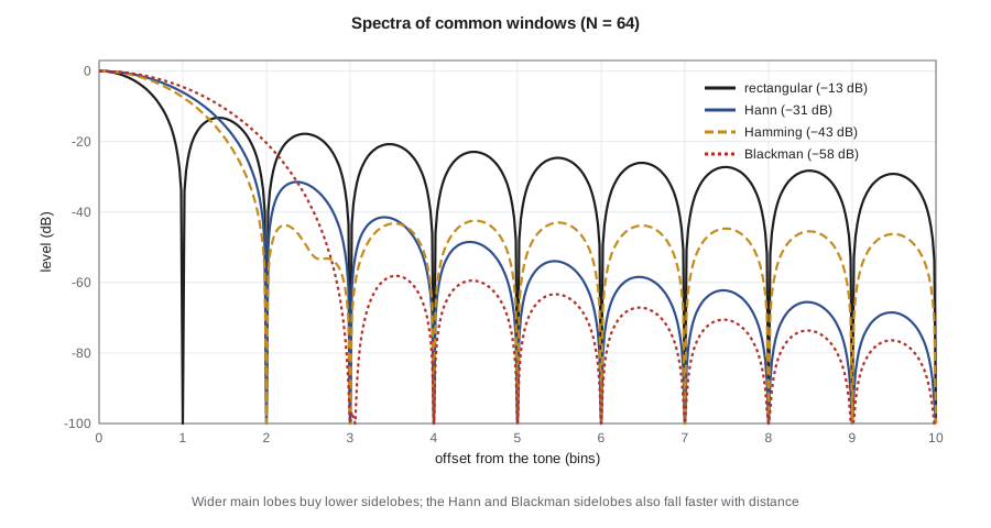
There is no best window, only a best window for a measurement. To measure the amplitude of a tone accurately when its frequency is not known, a flat-top window keeps the scalloping loss tiny. To find a weak tone near a strong one, a window with low sidelobes such as Blackman or a Kaiser window with a large β is right. To resolve two tones of similar size that are very close together, the rectangular or Hann window with its narrow main lobe is better. For general noise measurements, Hann is the usual compromise, and it is what Amara chooses for the spectrum monitor.
Zero padding
Appending zeros to a block before the DFT increases N and so decreases the bin spacing, but it adds no information. It interpolates the same windowed DTFT more finely. It makes peaks easier to locate and reduces the picket-fence effect, but it does not let two tones closer than about one main-lobe width be resolved; only a longer stretch of real data does that. Resolution is set by the observation time, about the reciprocal of the block duration times the window's main-lobe factor. A 32 ms block at 16 kHz cannot separate tones closer than about 31 Hz with a rectangular window, or 62 Hz with Hann, however many zeros are added.
Measuring noise: scaling and the periodogram
Tones and noise must be scaled differently. A tone's amplitude is read from its peak bin, divided by N times the coherent gain and doubled for a real signal. Noise has no single amplitude; it has a power spectral density (PSD), power per hertz. The squared magnitude of a windowed DFT, scaled correctly, is the periodogram, an estimate of the PSD. Its scaling must use the sum of w² rather than the sum of w, and the noise collected in each bin depends on the window's ENBW. Mixing up the two scalings is the most common error in spectrum measurement, and it typically misreads noise levels by 1.8 dB for a Hann window.
The periodogram has a surprising flaw: it does not get better with longer blocks. For noise, each bin's estimate has a standard deviation about equal to its mean, whatever N is; a longer block gives more bins, each just as noisy. The cure is averaging. Welch's method splits a long record into K overlapping segments, usually with 50 percent overlap, windows each, computes its periodogram and averages them. The relative standard deviation falls roughly as 1/√K, so 100 averages give spectral estimates good to about ±10 percent, or ±0.4 dB.
Worked problem
Reading the spectrum monitor
The spectrum monitor computes 256-point Hann-windowed DFTs at 16 kHz and averages 60 of them. A technician sees a peak at bin 8 and wants to know its frequency, the frequency uncertainty and how steady the noise floor estimate is.
Show solution
- \[\Delta f = \frac{16\,000}{256} = 62.5\ \text{Hz} \qquad f = 8 \times 62.5 = 500\ \text{Hz}\]
- The tone lies within about half a bin, ±31 Hz, unless the neighboring bins are used to interpolate the peak.
- \[\frac{\sigma}{\mu} \approx \frac{1}{\sqrt{60}} = 0.13 \;\Rightarrow\; \text{about } \pm 0.55\ \text{dB on the noise floor}\]
- \[T_{record} \approx 60 \times 128 / 16\,000 = 0.48\ \text{s with 50 \% overlap}\]
Answer: The peak is at 500 Hz, give or take 31 Hz, and the noise floor is good to about half a decibel after under half a second of data. The technician later finds the source: a cooling fan in a nearby building whose blade rate is close to 500 Hz.
import math, cmath, random
def fft(x):                                   # recursive radix-2 FFT (lesson 7 explains it)
    N = len(x)
    if N == 1: return list(x)
    E, O = fft(x[0::2]), fft(x[1::2])
    T = [cmath.exp(-2j * math.pi * k / N) * O[k] for k in range(N // 2)]
    return [E[k] + T[k] for k in range(N // 2)] + [E[k] - T[k] for k in range(N // 2)]
N = 256
wins = {
    "rectangular": [1.0] * N,
    "Hann": [0.5 - 0.5 * math.cos(2 * math.pi * n / N) for n in range(N)],
    "Hamming": [0.54 - 0.46 * math.cos(2 * math.pi * n / N) for n in range(N)],
    "Blackman": [0.42 - 0.5 * math.cos(2 * math.pi * n / N) + 0.08 * math.cos(4 * math.pi * n / N) for n in range(N)],
}
def W(w, bins):                               # window DTFT magnitude at a fractional bin offset
    return abs(sum(v * cmath.exp(-2j * math.pi * bins * n / N) for n, v in enumerate(w)))
for name, w in wins.items():
    s1, s2 = sum(w), sum(v * v for v in w)
    w0 = W(w, 0)
    side = max(W(w, b / 20) for b in range(20 if name == "rectangular" else 40 if name != "Blackman" else 60, 400)) / w0
    print(f"{name:11s} CG {s1/N:.2f}  ENBW {N*s2/s1**2:.2f} bins  scallop {-20*math.log10(W(w, 0.5)/w0):.2f} dB  highest sidelobe {20*math.log10(side):6.1f} dB")
random.seed(3); fs = 16000
noise = [random.gauss(0, 1) for _ in range(fs)]  # 1 s of white noise, variance 1
w = wins["Hann"]; s2 = sum(v * v for v in w)
for K in (1, 10, 100):
    segs = [noise[i * 128: i * 128 + N] for i in range(K)]
    psd = [0.0] * (N // 2)
    for sgm in segs:
        X = fft([a * b for a, b in zip(sgm, w)])
        for k in range(1, N // 2): psd[k] += 2 * abs(X[k]) ** 2 / (fs * s2) / K
    vals = psd[1:]
    m = sum(vals) / len(vals); sd = math.sqrt(sum((v - m) ** 2 for v in vals) / len(vals))
print(f"Welch K = {K:3d}: mean PSD {m:.3e} /Hz (theory {2/fs:.3e}), relative spread {sd/m:.2f}")rectangular CG 1.00 ENBW 1.00 bins scallop 3.92 dB highest sidelobe -13.3 dB Hann CG 0.50 ENBW 1.50 bins scallop 1.42 dB highest sidelobe -31.5 dB Hamming CG 0.54 ENBW 1.36 bins scallop 1.75 dB highest sidelobe -42.7 dB Blackman CG 0.42 ENBW 1.73 bins scallop 1.10 dB highest sidelobe -58.1 dB Welch K = 1: mean PSD 1.108e-04 /Hz (theory 1.250e-04), relative spread 0.98 Welch K = 10: mean PSD 1.232e-04 /Hz (theory 1.250e-04), relative spread 0.31 Welch K = 100: mean PSD 1.267e-04 /Hz (theory 1.250e-04), relative spread 0.09
The computed window figures match the table, which was drawn from the same definitions. The Welch results show the point of averaging: a single periodogram of white noise has a relative spread near 1, so individual bins scatter wildly about the true level of 2/f_s per hertz, while 10 averages bring the spread down to about 0.3 and 100 averages to roughly 0.1. The mean stays close to the theoretical value in every case, within the scatter expected for its K; what averaging changes is the confidence in each bin. The 50 percent overlap is why 100 segments of 256 samples fit into one second of data.
The spectrum monitor in the APS-2
Amara's spectrum monitor runs in the background at a low priority. Every few minutes it collects one second of 16 kHz microphone data, computes a 256-point Welch estimate with Hann windows and 50 percent overlap, converts the PSD to one-third-octave band levels in dB SPL using the calibration from lesson 3, and stores the result. A technician can request the latest spectra over the TLR-1 link. The data show at a glance whether a complaint about loud signals is caused by a real change in the street, such as construction or a new rooftop unit, or by a fault in the APS-2 itself, such as a damaged microphone whose high-frequency response has collapsed. The same machinery verifies the locator tone during the self-test, and lesson 12 replaces it there with a cheaper single-bin method.
Common mistakes
MistakeExpecting zero padding to resolve close tones.
InsteadZero padding interpolates; resolution depends on the length of real data and the window's main lobe.
MistakeScaling a noise spectrum with the tone formula.
InsteadUse the sum of w² (or ENBW) for PSD; the sum of w is for tone amplitude.
MistakeTrusting a single periodogram of noise.
InsteadEach bin has about 100 percent relative spread; average many segments with Welch's method.
MistakeMultiplying DFTs to filter without zero padding.
InsteadThat gives circular convolution; pad both to at least L + M − 1 samples for linear convolution.
Summary and key terms
- The N-point DFT samples the DTFT of a block at N frequencies spaced f_s/N and treats the block as one period of a periodic signal.
- DFT multiplication gives circular convolution; zero padding to L + M − 1 gives linear convolution.
- Tones between bins leak into all bins and are read low by the scalloping loss; windows trade main-lobe width for lower sidelobes.
- Coherent gain scales tone amplitudes; ENBW scales noise; choose the window for the measurement.
- Zero padding interpolates the spectrum but does not improve resolution, which depends on record length.
- The periodogram of noise does not improve with N; Welch averaging of K segments reduces the spread by about 1/√K.
- DFT bin
- One of the N equally spaced frequencies kf_s/N at which the DFT samples the spectrum.
- Leakage
- Spreading of a tone's energy into other bins when the block does not hold a whole number of cycles.
- Scalloping loss
- The reduction in a tone's apparent amplitude when it falls between bins.
- Window
- A taper applied to a data block before the DFT to control leakage.
- Equivalent noise bandwidth
- The width of an ideal rectangular filter that passes the same noise power as a DFT bin with a given window.
- Zero padding
- Appending zeros before a DFT to sample the spectrum more finely.
- Periodogram
- The scaled squared magnitude of a DFT, used as an estimate of power spectral density.
- Welch's method
- Averaging periodograms of overlapping windowed segments to reduce estimate variance.
Practice problems
Work each problem on paper first, then reveal the answer to check.
A 1024-point DFT runs at 48 kHz. What is the bin spacing, and which bin holds 3 kHz?
Show answer
46.875 Hz; bin 64.
Two sequences of length 100 and 29 are to be convolved with DFTs. What is the smallest N?
Show answer
128 (at least 128 samples, the next power of two above 100 + 29 − 1).
A tone is read with a Hann window exactly halfway between bins. How much low is it read?
Show answer
About 1.42 dB.
How many Welch averages give a relative spread of about 5 percent?
Show answer
1/√K = 0.05, K = 400.
A 64 ms record at 16 kHz is zero-padded from 1024 to 8192 points. Does resolution improve?
Show answer
No; bin spacing falls to 1.95 Hz but resolution stays about 15.6 Hz (rectangular) or 31 Hz (Hann).
Which window would you choose to measure a tone's amplitude within 0.1 dB when its frequency is unknown?
Show answer
A flat-top window, whose scalloping loss is negligible.
Lesson quiz · 5 questions
Score 60% or more to complete this lesson.
Create a free account to save your progress, take quizzes and earn a certificate.