
ELE-351 · Lesson 4 of 12 · 22 min
The z-transform and system functions
The z-transform does for discrete-time systems what the Laplace transform does for circuits: it turns convolution into multiplication and difference equations into algebra. ELE-250 introduced it, along with the idea that a filter's poles must lie inside the unit circle for stability. This lesson builds the working toolkit a DSP engineer uses every day: the region of convergence and what it says about causality and stability, the table of transform pairs and properties, the system function of a difference equation, inversion by partial fractions, and the connection between the positions of poles and zeros and how a system rings, decays or oscillates. The lesson ends with a practical use of all of it: a resonator that generates the APS-2's locator tone with two multiplies per sample.
Definition and region of convergence
The two-sided z-transform of a sequence x[n] is a power series in the complex variable z. It converges only for some values of z, and that set, the region of convergence (ROC), is part of the transform. The same algebraic expression can belong to two quite different sequences, distinguished only by their ROCs. The classic example is the exponential: aⁿu[n], which starts at n = 0 and runs to the right, and −aⁿu[−n − 1], which runs to the left, both have the transform 1/(1 − az⁻¹), the first for |z| > |a| and the second for |z| < |a|.
Three rules about the ROC carry most of the weight. The ROC never contains a pole, because the transform is infinite there. The ROC of a right-sided sequence, such as the impulse response of a causal system, is the outside of a circle through the outermost pole. And a sequence has a discrete-time Fourier transform exactly when its ROC includes the unit circle |z| = 1. For a causal LTI system, these combine into the rule from ELE-250: the system is stable if and only if all its poles are strictly inside the unit circle.
| Sequence | z-transform | ROC |
|---|---|---|
| δ[n] | 1 | all z |
| δ[n − k] | z⁻ᵏ | all z except 0 (k > 0) |
| u[n] | 1/(1 − z⁻¹) | |z| > 1 |
| aⁿu[n] | 1/(1 − az⁻¹) | |z| > |a| |
| naⁿu[n] | az⁻¹/(1 − az⁻¹)² | |z| > |a| |
| rⁿcos(ω₀n)u[n] | (1 − r cos ω₀ z⁻¹)/(1 − 2r cos ω₀ z⁻¹ + r²z⁻²) | |z| > r |
| rⁿsin(ω₀n)u[n] | (r sin ω₀ z⁻¹)/(1 − 2r cos ω₀ z⁻¹ + r²z⁻²) | |z| > r |
The properties that matter most in practice are short. Delaying a sequence by k samples multiplies its transform by z⁻ᵏ, so z⁻¹ is the unit delay of every block diagram. Convolution in time becomes multiplication of transforms, so cascaded systems multiply their system functions. Multiplying a sequence by aⁿ scales z, which moves every pole and zero radially by the factor a; this is how a filter is made more or less damped. Linearity lets sums be transformed term by term.
The system function
Taking the z-transform of the general difference equation of lesson 1, and using the delay property, gives the system function H(z) = Y(z)/X(z) as a ratio of polynomials in z⁻¹. The numerator coefficients are the feedforward coefficients b_k; the denominator coefficients are 1 and the feedback coefficients a_k. Factoring the polynomials gives the zeros, the roots of the numerator, and the poles, the roots of the denominator. A filter is completely specified, apart from an overall gain, by its poles and zeros.
An FIR filter has no denominator, so all its poles sit at the origin, and it is always stable. An IIR filter has poles elsewhere. For a filter with real coefficients, complex poles and zeros come in conjugate pairs, which is why IIR filters are almost always built from second-order sections, the biquads that appear throughout lessons 9 and 10. Each biquad holds one pair of poles and one pair of zeros.
Poles, zeros and behavior
The position of a pole tells how the corresponding part of the impulse response behaves. A real pole at p contributes pⁿ: a smooth decay if 0 < p < 1, an alternating decay if −1 < p < 0. A pair of complex poles at re^(±jθ) contributes a sinusoid of frequency θ rad/sample under an envelope rⁿ. The closer r is to 1, the slower the decay and the sharper the resonance in the frequency response. A pole exactly on the unit circle gives a sinusoid that neither grows nor decays, an oscillator. A pole outside the circle gives a growing response, an unstable system. Zeros shape the response by canceling frequencies: a zero on the unit circle at angle θ makes the frequency response exactly zero at ω = θ, which is how notch filters work.
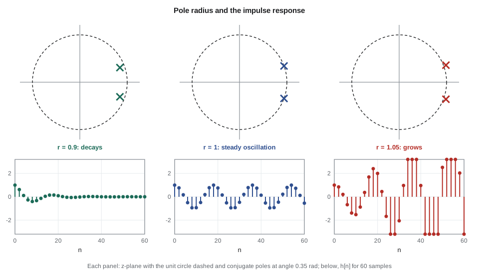
The time constant of a pole of radius r follows from rⁿ = e^(n ln r): the envelope falls by a factor e in about −1/ln r ≈ 1/(1 − r) samples. A useful equivalent links r to the 3 dB bandwidth of the resonance: for r close to 1, the bandwidth in hertz is about (1 − r)f_s/π. A biquad at 48 kHz with r = 0.999 therefore has a time constant of about 1000 samples, 21 ms, and a bandwidth of about 15 Hz.
Inverting the transform
Given a system function, the impulse response is found by inverting the transform. For rational transforms with distinct poles, partial fractions reduce the job to looking up the exponential pair. Write H(z) as a sum of first-order terms A_k/(1 − p_kz⁻¹); each coefficient is found by multiplying H(z) by (1 − p_kz⁻¹) and evaluating at z = p_k. With a causal ROC, each term inverts to A_kp_kⁿu[n]. Repeated poles give terms of the form npⁿ, and if the numerator degree is not less than the denominator degree, long division first removes a polynomial, which inverts to a short FIR part.
Worked problem
Partial-fraction inversion
A smoothing filter in the level meter has H(z) = 1/(1 − 1.5z⁻¹ + 0.56z⁻²). Find its poles, check stability and find h[n].
Show solution
- \[1 - 1.5z^{-1} + 0.56z^{-2} = \big(1 - 0.8z^{-1}\big)\big(1 - 0.7z^{-1}\big) \;\Rightarrow\; p_1 = 0.8, \; p_2 = 0.7\]
- Both poles are inside the unit circle, so the causal filter is stable.
- \[A_1 = \frac{1}{1 - 0.7/0.8} = 8 \qquad A_2 = \frac{1}{1 - 0.8/0.7} = -7\]
- \[h[n] = \big(8(0.8)^n - 7(0.7)^n\big)\,u[n]\]
Answer: The impulse response starts at h[0] = 1, rises to a peak of about 1.70 at n = 3 and then decays, dominated by the slower pole at 0.8. The code below checks the formula against the difference equation run sample by sample.
Long division gives another view: dividing the numerator polynomial by the denominator, term by term in powers of z⁻¹, produces h[0], h[1], h[2] and so on directly. It never gives a closed form, but it is exactly what running the difference equation with an impulse input does, and it is a good way to check a hand calculation.
A resonator as a tone generator
Place a pair of poles exactly on the unit circle at e^(±jω₀), with no input after the first sample, and the difference equation rings forever at frequency ω₀. That is a digital oscillator. With r = 1 the biquad recursion has only one multiply, by 2cos ω₀, and the right initial conditions set the amplitude and phase. For the APS-2's 880 Hz locator tone at 48 kHz, ω₀ = 0.11519 rad/sample and the coefficient is 2cos ω₀ = 1.98675.
The resonator is cheap, but Amara knows two weaknesses from experience. First, rounding errors are fed back every sample and never die away, because the poles are on the circle, so the amplitude slowly wanders; in floating point the drift is tiny over a 20 ms burst but measurable over hours. Second, the frequency depends on the stored coefficient, and rounding it to a fixed-point word shifts the frequency. Near ω₀ = 0 the shift is large, because cos ω₀ changes slowly there: a small change in the coefficient means a big change in the angle. The code shows the effect for a 16-bit coefficient. Lesson 10 returns to this coefficient sensitivity, which is the reason low-frequency IIR filters at high sample rates need care.
For the locator tone itself, the APS-2 does not need a free-running oscillator. Each burst lasts about 20 ms and repeats once a second, so Amara uses the lesson 1 observation that 600 samples hold exactly 11 cycles at 48 kHz: a 600-entry table generates the tone with no drift at all. The resonator remains useful where frequencies change at run time, for example in the self-test that sweeps a test tone through the speaker and microphone.
import math, struct
# 1. Partial-fraction result against the difference equation
a1, a2 = -1.5, 0.56
y1 = y2 = 0.0
for n in range(8):
    x = 1.0 if n == 0 else 0.0
    y = x - a1 * y1 - a2 * y2
    closed = 8 * 0.8 ** n - 7 * 0.7 ** n
    print(f"n={n}: recursion {y:8.5f}   formula {closed:8.5f}")
    y2, y1 = y1, y
# 2. Pole radius, time constant and bandwidth at 48 kHz
fs = 48000
for r in (0.99, 0.999, 0.9999):
    print(f"r = {r}: tau = {1000/(fs*(1-r)):7.2f} ms, 3 dB bandwidth about {(1-r)*fs/math.pi:6.2f} Hz")
# 3. 880 Hz resonator, exact coefficient against a 16-bit (Q2.14) coefficient
f0 = 880.0; w0 = 2 * math.pi * f0 / fs
def f32(v): return struct.unpack('f', struct.pack('f', v))[0]
for name, c in (("exact", 2 * math.cos(w0)), ("Q2.14", round(2 * math.cos(w0) * 16384) / 16384)):
    f_actual = fs * math.acos(c / 2) / (2 * math.pi)
    print(f"{name:6s} coefficient {c:.6f} -> tone at {f_actual:8.3f} Hz (error {round(f_actual - f0, 3) + 0.0:+.3f} Hz)")
c = f32(2 * math.cos(w0)); A = 1.0
y1, y2 = f32(-A * math.sin(w0)), f32(-A * math.sin(2 * w0))
peak = 0.0; peaks = []
for n in range(48000 * 10):          # ten seconds in single precision
    y = f32(f32(c * y1) - y2); y2, y1 = y1, y
    peak = max(peak, abs(y))
    if (n + 1) % (48000 * 2) == 0: peaks.append(peak); peak = 0.0
print("float32 resonator peak amplitude in each 2 s interval:", [round(p, 6) for p in peaks])n=0: recursion 1.00000 formula 1.00000 n=1: recursion 1.50000 formula 1.50000 n=2: recursion 1.69000 formula 1.69000 n=3: recursion 1.69500 formula 1.69500 n=4: recursion 1.59610 formula 1.59610 n=5: recursion 1.44495 formula 1.44495 n=6: recursion 1.27361 formula 1.27361 n=7: recursion 1.10124 formula 1.10124 r = 0.99: tau = 2.08 ms, 3 dB bandwidth about 152.79 Hz r = 0.999: tau = 20.83 ms, 3 dB bandwidth about 15.28 Hz r = 0.9999: tau = 208.33 ms, 3 dB bandwidth about 1.53 Hz exact coefficient 1.986746 -> tone at 880.000 Hz (error +0.000 Hz) Q2.14 coefficient 1.986755 -> tone at 879.673 Hz (error -0.327 Hz) float32 resonator peak amplitude in each 2 s interval: [1.000052, 1.000025, 1.000043, 1.000057, 1.000042]
The recursion and the closed form agree to every digit. The resonator results show both weaknesses: rounding the coefficient to 14 fractional bits moves the tone by a fraction of a hertz, harmless for a locator tone but a real problem for a narrow filter, and ten seconds of free running in single precision leaves the peak amplitude wandering by a few parts in a hundred thousand. Floating-point resonators are therefore fine for short bursts; fixed-point ones need amplitude correction or a table.
Stability and causality from the ROC
The ROC also answers a question that becomes important in lesson 5: can a system be both causal and stable? A causal system needs an ROC outside its outermost pole; a stable one needs the unit circle in its ROC. Both are possible together only if every pole is inside the circle. A system function with a pole outside the circle can still be stable, but only if it is non-causal, with an ROC that is a ring containing the unit circle. That is not useless: in off-line processing of recorded data, such as a filter run forward and backward over a stored file to cancel its phase, non-causal filters are perfectly practical. In real-time firmware like the APS-2, every filter must be causal, so every pole must be inside the circle, with margin for coefficient rounding.
Common mistakes
MistakeGiving a z-transform without its region of convergence.
InsteadThe same expression can describe a right-sided or a left-sided sequence; state the ROC or the causality assumption.
MistakeTesting stability by looking at zeros.
InsteadOnly poles decide stability; zeros can be anywhere, including outside the unit circle.
MistakeUsing a resonator with poles on the unit circle as a filter.
InsteadPoles on the circle give an oscillator; a filter needs r < 1 with a margin for rounding.
MistakeForgetting the conjugate pole when designing a real-coefficient resonance.
InsteadComplex poles of a real filter come in conjugate pairs; design them as a biquad.
Summary and key terms
- The z-transform turns convolution into multiplication; the ROC distinguishes sequences with the same algebraic transform.
- A causal system is stable exactly when all its poles are inside the unit circle.
- The system function is the ratio of feedforward to feedback polynomials; poles and zeros specify it up to a gain.
- Pole radius r sets decay (time constant about T/(1 − r)) and resonance bandwidth (about (1 − r)f_s/π); zeros on the circle null frequencies.
- Partial fractions invert rational transforms; long division or running the recursion checks the result.
- A biquad with poles on the circle is an oscillator; its frequency is sensitive to coefficient rounding, especially at low ω₀.
- Region of convergence
- The set of z for which the z-transform series converges.
- System function
- The ratio H(z) = Y(z)/X(z) for an LTI system.
- Pole
- A value of z where the system function becomes infinite; a root of its denominator.
- Zero
- A value of z where the system function is zero; a root of its numerator.
- Unit circle
- The circle |z| = 1, on which the z-transform reduces to the frequency response.
- Biquad
- A second-order section with two poles and two zeros.
- Partial fractions
- Writing a rational function as a sum of first-order terms to invert it.
- Digital resonator
- A biquad with poles near or on the unit circle that rings at a chosen frequency.
Practice problems
Work each problem on paper first, then reveal the answer to check.
Find the z-transform and ROC of x[n] = 0.5ⁿu[n] + 0.25ⁿu[n].
Show answer
1/(1 − 0.5z⁻¹) + 1/(1 − 0.25z⁻¹), |z| > 0.5.
A filter has poles at 0.95e^(±j0.3) and zeros at ±1. Is it stable? What are a₁ and a₂?
Show answer
Stable (r < 1); a₁ = −2(0.95)cos 0.3 = −1.815, a₂ = 0.9025.
Invert H(z) = 1/((1 − 0.5z⁻¹)(1 + 0.5z⁻¹)) for a causal system.
Show answer
A₁ = A₂ = 0.5: h[n] = 0.5(0.5)ⁿ + 0.5(−0.5)ⁿ, which is 0.25^(n/2) for even n and 0 for odd n.
What pole radius gives a 50 ms time constant at 16 kHz?
Show answer
1 − r = T/τ = 1/800, r = 0.99875.
Find the resonator coefficient for a 1 kHz tone at 16 kHz.
Show answer
2cos(π/8) = 1.84776.
Why can a filter with a pole at z = 1.2 still be useful off line?
Show answer
With an ROC |z| < 1.2 that includes the unit circle, it is stable but non-causal, which is fine for stored data.
Lesson quiz · 5 questions
Score 60% or more to complete this lesson.
Create a free account to save your progress, take quizzes and earn a certificate.