
DCE-450 · Lesson 6 of 12 · 25 min
Reliability engineering and availability
Commissioning proves that a data center works on the day it is tested. Reliability engineering asks a different question: how often will it fail over the next twenty years, and for how long each time? The answers shape design decisions worth millions of dollars, such as whether to add a fifth UPS module or a second utility feed, and they underpin the availability promises in customer contracts. This lesson introduces the vocabulary and the core calculations: failure rates and the bathtub curve, reliability and availability, mean time between failures and mean time to repair, how components combine in series and in parallel, k-of-n redundancy, and the common-cause failures that so often defeat redundancy in practice.
Reliability and availability are different
Reliability is the probability that an item performs its function without failure for a stated period under stated conditions. A UPS module with a reliability of 0.84 over one year has an 84 % chance of running the whole year without a failure. Availability is the fraction of time an item is able to perform its function. A system can be highly available but not very reliable, if it fails often but is repaired almost instantly, or reliable but poorly available, if it rarely fails but takes weeks to repair. Data center owners care about both: availability determines total downtime, while reliability determines how often customers experience an outage at all, and every outage, however short, can crash servers and corrupt data.
Failure rate and the bathtub curve
The failure rate, λ, is the number of failures per unit of operating time, often expressed in failures per million hours or as its reciprocal, the mean time between failures (MTBF). Over an equipment population's life, the failure rate typically follows the bathtub curve: a high but falling rate of early failures caused by manufacturing defects and installation errors (infant mortality), a long period of low and roughly constant random failures (useful life), and a rising rate as components wear out (wear-out). Commissioning is largely about flushing out infant mortality before the IT load arrives (Lessons 2 to 5), and maintenance and planned replacement are about staying out of the wear-out region (Lesson 8).
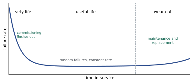
During the useful life, a constant failure rate means failures arrive at random, and the probability of surviving a period t without failure follows the exponential distribution:
A common misunderstanding is that MTBF is the expected life of an item. A UPS module with an MTBF of 50,000 hours (about 5.7 years) is not expected to last 5.7 years and then fail; under a constant failure rate, the chance it runs one year without failure is e^(−8760/50000) ≈ 0.84, and the chance it survives to its MTBF is only e^(−1) ≈ 37 %. MTBF describes how often failures occur across a population during useful life, not when wear-out begins.
Availability from MTBF and MTTR
If an item fails on average once every MTBF hours and takes on average MTTR (mean time to repair) hours to restore, its steady-state availability is:
Availability is often stated as a number of nines. Each extra nine divides annual downtime by ten:
| Availability | Nines | Downtime per year |
|---|---|---|
| 99 % | Two | 3.65 days |
| 99.9 % | Three | 8.8 hours |
| 99.99 % | Four | 53 minutes |
| 99.999 % | Five | 5.3 minutes |
| 99.9999 % | Six | 32 seconds |
MTTR includes far more than the repair itself: detecting the failure, diagnosing it, getting a technician and a spare part to site, the repair, testing and returning to service. For a UPS module with spares on site and a technician on call, MTTR may be a few hours; for a medium-voltage transformer without a spare, it may be months. Reducing MTTR, through spares, monitoring that pinpoints failures and trained staff, is often cheaper than improving MTBF.
Series systems
Components are in series, from a reliability point of view, when the failure of any one of them fails the system. A single power path from utility through switchgear, UPS and PDU to the rack is a series system. For independent components in series, availabilities (and reliabilities) multiply:
Because each factor is less than one, a series system is always less available than its weakest component. Adding more components in series, even very good ones, always lowers availability.
Parallel and k-of-n systems
Components are in parallel when the system works as long as at least one of them works. For two independent paths, each with availability A, the system fails only when both are down:
Data center equipment more often uses k-of-n redundancy: a UPS system of four modules where any three can carry the load (N+1, with N = 3), or five generators where any four are enough. The availability of a k-of-n system of identical, independent units is a binomial sum over the number of units working:
from math import comb, exp

HOURS = 8760

def availability(mtbf_h, mttr_h):
    return mtbf_h / (mtbf_h + mttr_h)

def downtime_min(a):
    return (1 - a) * HOURS * 60

def k_of_n(a, k, n):
    # probability that at least k of n identical, independent units are available
    return sum(comb(n, i) * a**i * (1 - a)**(n - i) for i in range(k, n + 1))

ups = availability(mtbf_h=50000, mttr_h=8)     # one UPS module
print(f"One UPS module:  A = {ups:.6f}, downtime {downtime_min(ups):6.1f} min/yr")
for k, n in [(3, 3), (3, 4), (3, 5)]:
    a = k_of_n(ups, k, n)
    print(f"{k}-of-{n} modules: unavailability {1 - a:.1e}, downtime {downtime_min(a):9.4f} min/yr")

# A simple power path in series: utility/generator source, switchgear, UPS system, PDU
path = {"source": 0.99995, "switchgear": 0.999995, "UPS 3-of-4": k_of_n(ups, 3, 4), "PDU": 0.99999}
series = 1.0
for a in path.values():
    series *= a
print(f"Series path:     A = {series:.6f}, downtime {downtime_min(series):6.1f} min/yr")
dual = 1 - (1 - series) ** 2
print(f"Two independent paths (2N): unavailability {1 - dual:.1e}, downtime {downtime_min(dual):.3f} min/yr")
beta = 0.05   # share of path failures that come from a common cause and take out both paths
u_cc = (1 - series) ** 2 + beta * (1 - series)
print(f"2N with 5 % common cause:   unavailability {u_cc:.1e}, downtime {u_cc * HOURS * 60:.2f} min/yr")

# Reliability over a year with a constant failure rate
lam = 1 / 50000
print(f"Chance one module runs a full year without failure: {exp(-lam * HOURS):.3f}")One UPS module: A = 0.999840, downtime 84.1 min/yr 3-of-3 modules: unavailability 4.8e-04, downtime 252.2073 min/yr 3-of-4 modules: unavailability 1.5e-07, downtime 0.0807 min/yr 3-of-5 modules: unavailability 4.1e-11, downtime 0.0000 min/yr Series path: A = 0.999935, downtime 34.2 min/yr Two independent paths (2N): unavailability 4.2e-09, downtime 0.002 min/yr 2N with 5 % common cause: unavailability 3.3e-06, downtime 1.71 min/yr Chance one module runs a full year without failure: 0.839
The output illustrates the main lessons. A single module with an MTBF of 50,000 hours and an MTTR of 8 hours is down about 84 minutes a year. Three modules with no redundancy (3-of-3) are worse than one, at over four hours a year, because any of three failures drops the load. Adding one redundant module (3-of-4) reduces expected downtime to under five seconds a year, and a second redundant module makes module failures practically irrelevant. Redundancy is enormously powerful, provided the redundant units fail independently.
Common-cause failures
The calculations above assume independence: one unit's failure tells you nothing about another's. Real failures often violate this. Two UPS systems may share a firmware bug, a maintenance error may be repeated on both paths, a single fire may damage both, a cooling failure may overheat both battery rooms, or a control system fault may command both to shut down. These common-cause failures take out redundant units together.
A simple way to account for them is the beta-factor model: a fraction β of each unit's failures is assumed to be common cause, affecting all redundant units at once. Even a small β dominates the result. In the output, two independent paths would be down about 0.002 minutes a year, but if just 5 % of path failures are common cause, expected downtime rises to about 1.7 minutes a year, almost a thousand times worse. Reliability data from operating data centers confirm this: most outages in redundant facilities are caused not by independent component failures but by common causes, human error and design flaws in the switching between redundant elements.
Designers reduce common-cause failures by diversity (different suppliers or technologies for redundant elements), physical separation (redundant paths in different rooms or fire compartments), independent controls, staggered maintenance and firmware updates, and procedures that prevent the same error being made on both sides.
Worked problem
Generators with failure to start
A site needs 4 of its 5 generators to carry the load. Each generator has a 1 % probability of failing to start on demand. Assuming independence, what is the probability that the site cannot carry its load when the utility fails? What if a 10 % share of start failures is common cause (for example contaminated fuel affecting all units)?
Show solution
- Probability all five start: 0.99⁵ = 0.951.
- Probability exactly four start: 5 × 0.99⁴ × 0.01 = 0.048.
- Probability at least four start: 0.951 + 0.048 = 0.99902, so the probability of insufficient generators is about 0.00098, roughly 1 in 1,000.
- With a beta factor of 0.1, the common-cause failure probability is about 0.1 × 0.01 = 0.001 per demand, which by itself is as large as all the independent combinations together. The total is about 0.002, or 1 in 500.
Answer: Independent failures give about a 1 in 1,000 chance of insufficient generators per utility outage; a modest common cause doubles it. Fuel quality testing and polishing, staggered maintenance and regular load testing (Lesson 8) attack the common cause directly.
Where the numbers come from
Failure rates and repair times come from manufacturers, from industry databases such as IEEE 493 (the Gold Book, Recommended Practice for the Design of Reliable Industrial and Commercial Power Systems), from insurers and from an operator's own maintenance records. All sources have limitations: manufacturer figures often exclude installation and operating errors; industry data are averaged across environments; and an operator's data may be thin for rare events. Reliability calculations are therefore best used to compare designs and to find weak points, rather than to predict a precise downtime figure.
Availability in contracts
Colocation and cloud providers promise availability in service level agreements (SLAs), typically for power and cooling at the rack, with credits paid when the promise is broken. SLA availability is measured from actual outages, not calculated, and the definitions matter: whether planned maintenance counts, whether a short dip counts, and at what point in the system availability is measured. Engineers should understand both the design availability calculated in this lesson and the measured availability reported against SLAs, and recognize that a facility designed for six nines can still suffer an outage in its first year.
Common mistakes
MistakeTreating MTBF as expected life.
InsteadMTBF is a population failure rate during useful life; most units fail before or after it.
MistakeAdding non-redundant components and expecting higher availability.
InsteadComponents in series always lower availability.
MistakeAssuming redundant units fail independently.
InsteadModel common causes and design separation and diversity to reduce them.
MistakeCounting only repair time in MTTR.
InsteadInclude detection, diagnosis, travel, parts, repair and testing.
MistakeQuoting calculated availability as a prediction.
InsteadUse calculations to compare designs and find weak points.
Summary and key terms
- Reliability is the probability of no failure over a period; availability is the fraction of time working.
- Failure rates follow the bathtub curve; commissioning targets early failures and maintenance targets wear-out.
- Under a constant failure rate, R(t) = e^(−λt) and MTBF = 1/λ.
- Availability = MTBF / (MTBF + MTTR); each nine divides downtime by ten.
- Series availabilities multiply; parallel and k-of-n redundancy raise availability dramatically.
- Common-cause failures usually dominate redundant systems.
- Reliability numbers are best for comparing designs, not exact predictions.
- Reliability
- The probability of performing without failure for a stated period.
- Availability
- The fraction of time an item can perform its function.
- Failure rate
- Failures per unit of operating time.
- MTBF
- Mean time between failures, the reciprocal of a constant failure rate.
- MTTR
- Mean time to repair, from failure to return to service.
- Bathtub curve
- The typical pattern of failure rate over equipment life.
- Series system
- A system that fails if any component fails.
- k-of-n redundancy
- A system that works if at least k of n units work.
- Common-cause failure
- A single cause that fails several redundant units together.
- Beta factor
- The fraction of failures assumed to be common cause.
Practice problems
Work each problem on paper first, then reveal the answer to check.
An item has MTBF 20,000 h and MTTR 10 h. What is its availability?
Show answer
20,000 / 20,010 = 0.9995.
How much downtime per year does 99.99 % availability allow?
Show answer
About 53 minutes.
What is the probability that an item with MTBF 50,000 h survives to 50,000 h?
Show answer
e^(−1) ≈ 37 %.
Three components in series have availabilities 0.999, 0.9995 and 0.9999. What is the system availability?
Show answer
About 0.99840.
Two parallel paths each have A = 0.999. What is the system availability, assuming independence?
Show answer
1 − 0.001² = 0.999999.
From the output, why is 3-of-3 worse than a single module?
Show answer
Any of three module failures drops the load.
From the output, how much does a 5 % common cause increase 2N downtime?
Show answer
From about 0.002 to about 1.7 minutes a year.
List three ways to reduce common-cause failures.
Show answer
For example: diversity, physical separation, independent controls, staggered maintenance and firmware updates.
Name four components of MTTR.
Show answer
Detection, diagnosis, travel and parts, repair, testing and return to service.
Why is measured SLA availability different from calculated availability?
Show answer
It comes from actual outages and depends on contract definitions; calculations are model estimates.
Lesson quiz · 5 questions
Score 60% or more to complete this lesson.
Create a free account to save your progress, take quizzes and earn a certificate.