Cabling for AI and high-performance computing clusters

Training large AI models links thousands of accelerators (GPUs or similar processors) into a single machine, exchanging data among them constantly. The network that does this, the back-end or compute fabric, needs several times more bandwidth per server than a conventional data center network, and every accelerator has its own high-speed port. The result is a cabling plant with an order of magnitude more fiber than an enterprise hall of the same floor area, concentrated around racks that each draw tens or hundreds of kilowatts. This lesson explains the networks in an AI cluster, the rail-optimized topology, how to count links and fibers, where to place switches, and the practical limits of pathways, cable management and installation at this scale.

The networks in an AI cluster

A typical AI training server holds eight accelerators and connects to several separate networks:

• Back-end (compute) fabric: one high-speed port per accelerator, at 400 Gb/s or 800 Gb/s, using InfiniBand or Ethernet with RDMA. This network carries the collective operations, such as all-reduce, that synchronize training. It is built non-blocking and must have very low loss and latency.
• Scale-up network: inside the server or rack, accelerators connect directly to each other at even higher bandwidth through proprietary links such as NVLink, often over copper. Rack-scale systems extend this across a whole rack of 36 to 72 accelerators.
• Front-end network: a conventional Ethernet network at 100 to 400 Gb/s per server, for storage access, data loading, users and management of jobs.
• Storage network: sometimes separate, connecting servers to high-performance file systems.
• Out-of-band management: Category 6A copper to each server's management controller, PDUs and switches (Lesson 3).

The back-end fabric dominates the cabling: with eight 400G ports per server, plus front-end and management connections, a single server may need 80 or more fibers.

Rail-optimized topology

In a rail-optimized fabric, the accelerators in each server are numbered 1 to 8, and all accelerators with the same number, across a group of servers, connect to the same leaf switch (or set of leaves), called a rail. Accelerator 1 of every server in the group goes to rail 1, accelerator 2 to rail 2, and so on. Collective operations mostly exchange data between accelerators with the same number, so most traffic stays within one rail leaf, one switch hop, and the spine layer carries the rest.

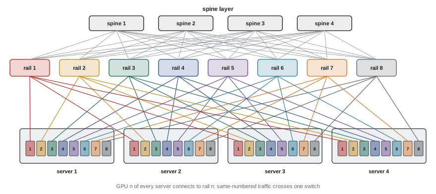
The cabling consequence is that each server sends one link to each of eight different leaf switches, so its cables spread across the network racks rather than going to a single top-of-rack switch. Top-of-rack switching is not used for the back-end fabric; leaves are placed in network racks at the end or middle of each row, or in a central network row.

Clusters are built in units, often called scalable units or pods, of a fixed number of servers (for example 32 servers and 256 accelerators) with their rail leaves, so that a design can be repeated row by row. A pod might be one row of cabinets with a network rack in the middle.

Counting links and fibers

The first step in designing an AI cluster plant is to count the links between each pair of locations: server cabinets to leaf racks, and leaf racks to spine racks. For a non-blocking two-tier fabric, the leaf-to-spine bandwidth equals the server-to-leaf bandwidth, so the link counts are similar.

import math

# Back-end (compute) fabric for an AI cluster, rail-optimized, two tiers.
servers = 512
gpus_per_server = 8
fibres_per_link = 8          # 400G DR4 at every NIC, 800G 2xDR4 on switches
trunk_fibres = 144           # fibres per trunk cable
trunk_diam_mm = 11.0
cabinets_per_row = 16
servers_per_cabinet = 2      # power density limits servers per cabinet

gpus = servers * gpus_per_server
rows = servers // (servers_per_cabinet * cabinets_per_row)
print(f"GPUs {gpus}, server cabinets {servers // servers_per_cabinet}, rows {rows}")

# Tier 1: every GPU NIC to a rail leaf (one 400G link each)
leaf_links = gpus
# Tier 2: leaf to spine, non-blocking, counted in 400G equivalents
spine_links = gpus

for name, links in (("server-leaf", leaf_links), ("leaf-spine", spine_links)):
    fibres = links * fibres_per_link
    trunks = math.ceil(fibres / trunk_fibres)
    area_cm2 = trunks * math.pi * (trunk_diam_mm / 20) ** 2
    print(f"{name:12s} links {links:5d}  fibres {fibres:6d}  trunks {trunks:4d}  cable area {area_cm2:6.0f} cm2")

per_row = leaf_links // rows
print(f"server-leaf fibres leaving each row: {per_row * fibres_per_link}")

GPUs 4096, server cabinets 256, rows 16
server-leaf  links  4096  fibers  32768  trunks  228  cable area    217 cm2
leaf-spine   links  4096  fibers  32768  trunks  228  cable area    217 cm2
server-leaf fibers leaving each row: 2048

Each tier needs about 33,000 fibers. The leaf-to-spine links travel further, from every row to the spine racks, and they all converge on one area, which is the hardest part of the pathway design. The total, with front-end, storage and management cabling and spare capacity, approaches 100,000 fibers for a cluster of this size, and current clusters are many times larger.

Placing the switches

Link length decides which media can be used, and in AI clusters the choice of switch location balances several pressures:

• Short links allow cheaper optics or copper: multimode SR optics reach only 50 m to 100 m, and passive copper only a meter or two.
• Power density limits how many servers fit in a cabinet, spreading them over more floor and lengthening links. A cabinet of air-cooled 8-accelerator servers might hold only one or two servers at 40 kW or more; liquid-cooled rack-scale systems concentrate 100 kW or more in a rack.
• Network racks themselves have high power: a rack of 51.2 Tb/s switches with their optics can draw 20 kW or more.
• Spine racks gather links from the whole cluster, so their location sets the longest links. A central spine location minimizes the maximum length.

Most large clusters now use single-mode DR optics for the back-end fabric, so that 500 m reach removes length as a constraint within a building, and switch placement can follow power and cooling. Multimode is used where all links stay within a row or two.

Pathways at AI scale

The cable volumes from the code example, over 200 cm² of trunk cable per tier, concentrate near the spine racks, where every row's trunks arrive. Several practices keep this manageable:

• Use high fiber-count trunks with small diameters (rollable ribbon, 200 µm fiber) instead of many small cables, reducing volume and installation time.
• Run trunks in dedicated overhead fiber pathways (such as enclosed fiber raceway or wide wire-basket trays), separated from power busway and liquid-cooling pipework.
• Plan levels: power busway, cooling pipes, copper trays and fiber trays each at their own height, with clear crossing points (Lesson 8).
• Size pathways for at least two generations: the next cluster generation may double the fibers per accelerator.
• Keep fiber trays away from liquid-cooling manifolds and below-cabinet leak paths, and avoid routing fiber beneath overhead pipes where a leak would drip onto it.

Liquid cooling also changes the cabinet itself: manifolds, hoses and coolant distribution units occupy the rear of rack-scale systems, where cables traditionally ran. Cable entry, slack storage and patch panel locations must be agreed with the cooling design early.

Structured or direct cabling?

Two approaches compete for the server-to-leaf links:

• Direct cabling: a cord runs from each server port directly to the leaf switch port, often an AOC or long single-mode patch cord. It has the fewest connections and lowest loss, and is quick for a cluster installed all at once. But thousands of long cords are hard to manage, trace and replace.
• Structured cabling: MPO trunks run from a panel in each server cabinet to panels in the network rack, and short cords connect equipment to panels at each end. It adds two mated connections (about 0.7 dB with low-loss MPO), but cords are short, faults are easy to isolate, and racks can be moved or re-cabled without disturbing the trunk.

For large clusters with long service lives, structured cabling is usually preferred, and many operators use pre-terminated trunks built to length from a 3D model of the hall, delivered labeled and tested from the factory. This shortens on-site work, which matters when a cluster worth hundreds of millions must be operational in weeks.

Installation and acceptance at scale

Installing 100,000 fibers in weeks needs industrial methods:

• Pre-terminated, factory-tested trunks and cassettes, with labels printed from the design database (Lesson 10).
• Installation by pod, with each pod tested and handed over as it is completed, so the network team can start bringing it up while the next is installed.
• Automated MPO inspection and testing, with results uploaded directly to the records system.
• Link verification by the network itself: once switches are installed, the fabric management software checks that each port is connected to the expected neighbor (using LLDP or the fabric's own discovery). Cabling errors, such as a server port on the wrong rail, are found and fixed before training jobs run.

A single miscabled link in a rail-optimized fabric may not stop the cluster but can slow every job that uses it, so verification of the actual connections against the design is as important as loss testing.