Testing, certification and troubleshooting

Lesson 3 described copper certification and Lesson 6 introduced fiber testing tiers and the inspect-and-clean rule. This lesson goes further: how loss measurements are referenced and why the method changes the result, how to read an OTDR trace, how to write a test specification that a contractor can price and an owner can enforce, and how to troubleshoot links that fail at acceptance or in service. A cabling plant is accepted on its test results, and those results are its warranty, its baseline for future troubleshooting and the evidence that the design was built.

Why referencing matters

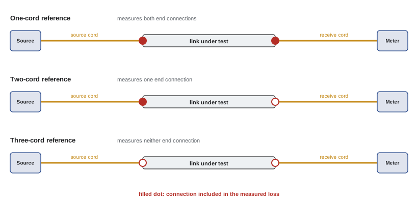
An optical loss test set (OLTS) measures power with a light source at one end and a power meter at the other. Before testing, the tester is set to zero (referenced) with test cords, so that the result shows only the loss of the link under test. The way the reference is taken decides which connections are included in the result:

• One-cord reference (TIA Method B, IEC Method 1): the source cord is connected directly to the meter for the reference. When the link is inserted, the result includes both end connections and the fiber. This is the preferred method for testing installed links, because the connections at both patch panels are part of the channel.
• Two-cord reference (Method A, IEC Method 2): the reference includes one connection, so the result includes only one end connection.
• Three-cord reference (Method C, IEC Method 3): the reference includes both, so the result shows only the fiber and any internal connections.

The test cords themselves must be reference-grade: their connectors have tighter tolerances than ordinary patch cords, so that the measured loss reflects the link and not the cords. They wear with use and should be checked against each other regularly and replaced when they exceed their limit (often 0.1 dB to 0.2 dB for a reference connection).

Encircled flux

A multimode light source that fills all the modes of the fiber makes connections look worse, because high-order modes are lost first at a misaligned joint; a source that fills only low-order modes makes them look better. To make results repeatable, standards require multimode sources to meet the encircled flux (EF) launch condition (IEC 61280-4-1), usually achieved with a mode controller on the source cord. Results taken without EF control can vary by tenths of a decibel per connection, enough to pass or fail a link.

Setting pass/fail limits

Each link is judged against a limit. Two approaches are used:

• Application limits: the maximum channel loss allowed by the optics the link will carry, such as 1.9 dB for 400GBASE-SR8 on OM4 or 3.0 dB for 400GBASE-DR4. The link passes if it will work for that application.
• Link (installation) limits: the loss calculated from the actual design, using maximum values for each component. A link with two connections and 80 m of OM4 might have a limit of \(2 \times 0.35 + 0.08 \times 3.0 = 0.94\) dB with low-loss connectors. This checks workmanship: a link that is well below the application limit but well above its design value shows something is wrong.

A good test specification requires both: every link must meet its calculated design limit, which ensures it also meets the application limits with margin.

Reading an OTDR trace

An optical time-domain reflectometer sends short pulses into one end of a fiber and records the light that returns over time. Two kinds of light return: Rayleigh backscatter from the glass itself, a weak continuous signal that falls with distance as the fiber attenuates both the outgoing pulse and the returning light; and Fresnel reflections, sharp spikes from connectors, mechanical splices and the far end. The trace plots returned power in dB against distance, calculated from the time and the fiber's group index.

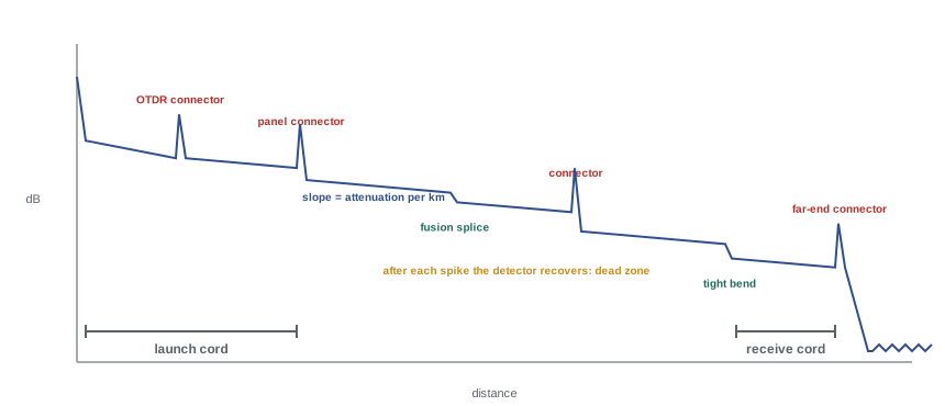
Key features of a trace:

• Slope: the attenuation of the fiber, in dB/km. The displayed backscatter falls at the one-way rate, because OTDR software divides the round-trip loss by two.
• Non-reflective events: steps down with no spike, from fusion splices and bends. A bend loses more at longer wavelengths, so comparing traces at 1,310 nm and 1,550 nm distinguishes a bend from a splice.
• Reflective events: spikes with a step, from connectors and mechanical splices. The height of the spike gives the reflectance.
• Dead zones: after a strong reflection the detector is saturated for a short distance. The event dead zone (about 1 m on a good instrument) is the minimum distance to see a second event; the attenuation dead zone (several meters) is the distance before loss can be measured again. Launch and receive cords, typically 30 m to 150 m for data center links, move the first and last connectors of the link out of the dead zones so their loss can be measured.
• Gainers: a splice between fibers with different backscatter coefficients can appear as a gain in one direction and an exaggerated loss in the other. Testing from both ends and averaging gives the true loss.

import numpy as np

# Synthetic OTDR trace of a single-mode link at 1310 nm, sampled every 1 m.
rng = np.random.default_rng(7)
x = np.arange(0, 1400)                       # metres from the OTDR
alpha = 0.35 / 1000                          # dB per metre, one way
events = {150: 0.25, 480: 0.08, 900: 0.45, 1250: 0.30}   # position: loss in dB

trace = -2 * alpha * x                       # backscatter falls at twice the one-way loss
for pos, loss in events.items():
    trace[x >= pos] -= 2 * loss
trace += rng.normal(0, 0.004, x.size)        # receiver noise

# Fit a straight line to each section and measure the step at each event.
found = []
d = trace[5:] - trace[:-5]                   # change over 5 m
expected = -2 * alpha * 5
cand = np.where(d < expected - 0.06)[0]
groups = np.split(cand, np.where(np.diff(cand) > 3)[0] + 1)
for g in groups:
    if g.size == 0:
        continue
    p = int(g.mean()) + 3
    before = np.polyfit(x[p - 60:p - 5], trace[p - 60:p - 5], 1)
    after = np.polyfit(x[p + 5:p + 60], trace[p + 5:p + 60], 1)
    step = np.polyval(before, p) - np.polyval(after, p)
    found.append((p, step / 2))
for p, loss in found:
    print(f"event near {p:5d} m   loss {loss:.2f} dB")
slope = -np.polyfit(x[200:470], trace[200:470], 1)[0] / 2 * 1000
print(f"fibre attenuation from slope: {slope:.2f} dB/km")

event near   150 m   loss 0.25 dB
event near   480 m   loss 0.08 dB
event near   900 m   loss 0.45 dB
event near  1250 m   loss 0.30 dB
fiber attenuation from slope: 0.35 dB/km

In a data center, OTDR testing is most useful on backbone and campus links, on links that fail loss testing, and for finding where a fault is. On very short links with closely spaced connectors, the dead zones make it hard to separate events, and high-resolution instruments with short pulses are needed.

Writing a test specification

A cabling contract should state exactly what testing is required, so that contractors price the same work and the owner can reject unacceptable results:

• Scope: 100% of links, by type, with Tier 1 loss testing of all fiber and OTDR testing of backbone and outside plant links, plus copper certification of all twisted-pair links.
• Methods: the reference method (one-cord), encircled flux for multimode, wavelengths (850 and 1,300 nm multimode; 1,310 and 1,550 nm single-mode), and bidirectional testing where required.
• Limits: the design-based limit for each link, and the application limits to be reported.
• Inspection: end-face inspection of every connector against IEC 61300-3-35, with images saved.
• Equipment: calibrated instruments, reference-grade cords, and records of reference checks.
• Records: native tester files plus a summary report, named with the link identifiers from the labeling scheme (Lesson 10), delivered before acceptance.
• Retesting: any repaired link retested completely, and any link failing for an unknown reason investigated with OTDR.

The owner or an independent engineer should witness a sample of tests and spot-check the records. Missing or doctored results are not rare, and a sample retest by a separate party is a strong deterrent.

Troubleshooting

Most failures at acceptance and in service have a short list of causes. A systematic approach finds them quickly:

• Start with the simplest checks: is the link connected end to end, with correct polarity? A visual fault locator (VFL), a red 650 nm laser, shows breaks and tight bends as a glow through the jacket and confirms continuity and polarity over short links.
• Inspect and clean every connector in the path, including the transceiver ports and test cords. Contamination causes the majority of fiber faults.
• Compare with the design limit. A link a few tenths of a decibel high usually has a dirty or damaged connector; a link several decibels high has a break, a bad splice, a crushed cable or the wrong fiber type in the path.
• Use the OTDR to locate the problem along the link, testing from both ends if a gainer or the dead zone hides it.
• Check for mixed fiber types: a multimode cord in a single-mode link, or OM2 (62.5 µm in older sites, or 50 µm with lower bandwidth) mixed with OM4, causes high loss or errors.

Using the equipment's own monitoring

Most modules report their transmit and receive optical power, temperature and bias current through digital optical monitoring (DOM, also called digital diagnostic monitoring). Network monitoring systems collect these values, and a link whose receive power is falling over weeks, or is near the receiver sensitivity, can be cleaned or repaired before it fails. FEC statistics give an even earlier warning: the pre-FEC bit error ratio rises as margin is lost.