Attention and transformers

The transformer, introduced by Ashish Vaswani and seven colleagues at Google in the 2017 paper Attention Is All You Need, is the architecture behind nearly every large language model, most state-of-the-art speech and vision systems, protein structure predictors and much else. It drops recurrence and convolution entirely and builds everything from attention, a mechanism that lets each position in a sequence gather information directly from every other position, combined with the feedforward layers, residual connections and normalization of earlier lessons. This lesson derives scaled dot-product attention, implements it with a causal mask, explains multi-head attention and positional encodings including rotary embeddings, assembles the transformer block, and works through its computational costs, including the quadratic cost of attention and the key-value cache used during generation. AI-340 covers the transformer's use in language, AI-410 large language models, and AI-350 vision transformers.

Attention as soft lookup

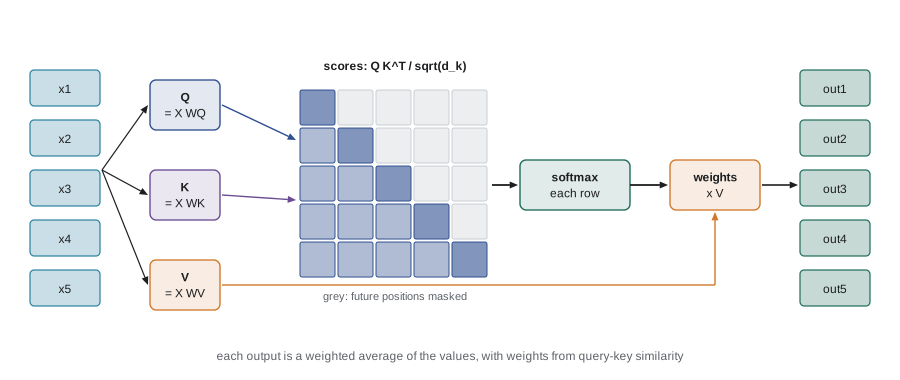
Attention can be understood as a differentiable dictionary lookup. A query vector is compared with a set of key vectors, each comparison produces a score, the scores are turned into weights by a softmax, and the result is the weighted average of the value vectors associated with the keys. A hard lookup would return the single value whose key matches; attention returns a blend, weighted toward the best matches, and because every step is differentiable the network can learn what to put in the queries, keys and values. Bahdanau attention (lesson 7) scored query-key pairs with a small network; Minh-Thang Luong and colleagues (2015) used dot products, which are cheaper and map well onto matrix hardware.

In self-attention, the queries, keys and values all come from the same sequence. Each position's representation \(\mathbf{x}_t\) is projected three ways, \(\mathbf{q}_t = W_Q^{\top}\mathbf{x}_t\), \(\mathbf{k}_t = W_K^{\top}\mathbf{x}_t\), \(\mathbf{v}_t = W_V^{\top}\mathbf{x}_t\), and with all positions stacked as rows of matrices Q, K and V, scaled dot-product attention is

where the softmax is applied to each row. Row t of \(QK^{\top}\) holds the similarity of position t's query with every key; after the softmax it is a probability distribution saying where position t looks, and multiplying by V gathers the corresponding values. Every position is connected to every other in a single step, so the path length between any two positions is 1, against T for an RNN. And all positions are computed at once with matrix products, which GPUs do extremely well.

# Scaled dot-product self-attention with a causal mask, from scratch in NumPy.
import numpy as np
rng = np.random.default_rng(466)
T, d_model, d_k = 5, 8, 4
X = rng.normal(size=(T, d_model))                       # 5 token representations
Wq, Wk, Wv = (rng.normal(0, d_model ** -0.5, (d_model, d_k)) for _ in range(3))
Q, K, V = X @ Wq, X @ Wk, X @ Wv
def attention(Q, K, V, causal):
    scores = Q @ K.T / np.sqrt(K.shape[1])               # T x T similarity of every query with every key
    if causal:
        scores = np.where(np.triu(np.ones_like(scores), 1) == 1, -np.inf, scores)   # hide the future
    scores -= scores.max(axis=1, keepdims=True)
    A = np.exp(scores); A /= A.sum(axis=1, keepdims=True)   # each row is a probability distribution
    return A @ V, A
out, A = attention(Q, K, V, causal=True)
np.set_printoptions(precision=3, suppress=True)
print("causal attention weights (row = query position, column = key position):")
print(A)
print("rows sum to 1:", np.allclose(A.sum(1), 1), "  output shape:", out.shape)
# permuting the tokens without a causal mask just permutes the outputs: attention has no notion of order
perm = rng.permutation(T)
o1, _ = attention(Q, K, V, causal=False); o2, _ = attention(Q[perm], K[perm], V[perm], causal=False)
print("without positions, self-attention is permutation-equivariant:", np.allclose(o1[perm], o2))

causal attention weights (row = query position, column = key position):
[[1.    0.    0.    0.    0.   ]
 [0.772 0.228 0.    0.    0.   ]
 [0.447 0.405 0.148 0.    0.   ]
 [0.03  0.328 0.282 0.36  0.   ]
 [0.356 0.339 0.078 0.14  0.088]]
rows sum to 1: True   output shape: (5, 4)
without positions, self-attention is permutation-equivariant: True

Why scale by the square root of the dimension

If the entries of \(\mathbf{q}\) and \(\mathbf{k}\) are independent with mean 0 and variance 1, their dot product is a sum of \(d_k\) terms of variance 1, so it has variance \(d_k\). With \(d_k = 64\) the scores have standard deviation 8, and the softmax of such widely spread scores is nearly one-hot: one key gets almost all the weight and the gradients with respect to the others vanish, the same saturation problem as with sigmoids. Dividing by \(\sqrt{d_k}\) restores unit variance and keeps the softmax in a regime where gradients flow. Later work sometimes normalizes queries and keys directly (QK-norm) to keep scores bounded during long training runs.

# Why divide by sqrt(d_k): dot products of random unit-variance vectors have variance d_k.
import numpy as np
rng = np.random.default_rng(466)
for d in (4, 64, 512):
    q = rng.normal(size=(5000, d)); k = rng.normal(size=(5000, d))
    dots = np.sum(q * k, axis=1)
    s = rng.normal(size=(2000, 16, d)) @ rng.normal(size=(d,))        # 16 keys per query
    def peak(scores):
        e = np.exp(scores - scores.max(1, keepdims=True)); return (e / e.sum(1, keepdims=True)).max(1).mean()
    print(f"d_k = {d:3}: std of q.k = {dots.std():6.2f} (sqrt(d) = {np.sqrt(d):5.2f});  "
          f"mean largest softmax weight over 16 keys: unscaled {peak(s):.3f}, scaled {peak(s / np.sqrt(d)):.3f}")

d_k =   4: std of q.k =   2.00 (sqrt(d) =  2.00);  mean largest softmax weight over 16 keys: unscaled 0.514, scaled 0.281
d_k =  64: std of q.k =   8.01 (sqrt(d) =  8.00);  mean largest softmax weight over 16 keys: unscaled 0.829, scaled 0.220
d_k = 512: std of q.k =  22.81 (sqrt(d) = 22.63);  mean largest softmax weight over 16 keys: unscaled 0.938, scaled 0.232

Causal masking

A language model predicts each token from the ones before it. During training the whole sequence is processed at once, so position t must be prevented from looking at positions after t, or the model would learn to copy the answer. Setting the scores above the diagonal to \(-\infty\) before the softmax gives those positions zero weight, as in the program's output, whose upper triangle is zero. This causal mask is what makes a decoder-only transformer such as GPT a valid autoregressive model while still training on all positions of a sequence in parallel. Encoders such as BERT omit the mask, so every position sees the whole input, which suits understanding tasks but not left-to-right generation. Padding masks similarly hide padding tokens in batches of unequal-length sequences.

Multi-head attention

One attention distribution per position is limiting: a word may need to attend to its subject for agreement, to a nearby adjective for meaning and to a distant antecedent for reference, all at once. Multi-head attention runs h attention operations in parallel, each with its own projections into a smaller dimension \(d_k = d/h\), concatenates their outputs and applies an output projection \(W_O\):

Because each head works in dimension d/h, the total cost is about the same as one full-width head. Different heads learn different patterns; interpretability studies have found heads that attend to the previous token, to matching brackets, to syntactic relations, and induction heads that look for an earlier occurrence of the current token and copy what followed it (Catherine Olsson and colleagues at Anthropic, 2022), a mechanism linked to in-context learning. To reduce memory during generation, multi-query attention (Noam Shazeer, 2019) shares one key and value projection across all heads, and grouped-query attention (Joshua Ainslie and colleagues, 2023) shares them within groups of heads; most recent large language models use grouped-query attention.

Positional information

Attention by itself is permutation-equivariant: shuffle the input positions and the outputs are shuffled the same way, as the first program verified. Word order must therefore be injected explicitly. The original transformer added fixed sinusoidal positional encodings to the input embeddings, with dimension pairs oscillating at geometrically spaced frequencies so that each position has a unique pattern and nearby positions have similar ones. BERT and GPT-2 instead learned a position embedding vector for each position up to a maximum length, which cannot extend beyond that length.

Rotary position embedding (RoPE; Jianlin Su and colleagues, 2021) applies position inside attention rather than to the input. It rotates each consecutive pair of query and key dimensions by an angle proportional to the position, with a different frequency for each pair. Because rotations compose, the dot product of a query rotated by position m and a key rotated by position n depends only on the offset m − n, so attention scores are a function of relative position. RoPE is used in most open large language models, including the Llama, Mistral and Qwen families, and variants that rescale its frequencies are used to extend context length after training. ALiBi (Ofir Press and colleagues, 2022) instead adds a penalty to the score proportional to distance.

# Sinusoidal positional encodings and rotary embeddings (RoPE): RoPE scores depend only on relative position.
import numpy as np
def sinusoidal(T, d):
    pos = np.arange(T)[:, None]; i = np.arange(d // 2)[None, :]
    ang = pos / 10000 ** (2 * i / d)
    pe = np.zeros((T, d)); pe[:, 0::2] = np.sin(ang); pe[:, 1::2] = np.cos(ang)
    return pe
pe = sinusoidal(50, 16)
print("sinusoidal PE, positions 0 and 1, first 6 dimensions:")
print(np.round(pe[:2, :6], 3))
def rope(x, pos):                                    # rotate each pair of dimensions by pos * frequency
    d = x.shape[-1]; freq = 1 / 10000 ** (np.arange(d // 2) * 2 / d)
    ang = pos * freq; c, s = np.cos(ang), np.sin(ang)
    x1, x2 = x[0::2], x[1::2]
    out = np.empty_like(x); out[0::2] = x1 * c - x2 * s; out[1::2] = x1 * s + x2 * c
    return out
rng = np.random.default_rng(466)
q, k = rng.normal(size=16), rng.normal(size=16)
for m, n in ((3, 1), (10, 8), (42, 40)):             # all have offset m - n = 2
    print(f"query at {m:2}, key at {n:2}: RoPE score {rope(q, m) @ rope(k, n):.6f}")

sinusoidal PE, positions 0 and 1, first 6 dimensions:
[[0.    1.    0.    1.    0.    1.   ]
 [0.841 0.54  0.311 0.95  0.1   0.995]]
query at  3, key at  1: RoPE score -2.963328
query at 10, key at  8: RoPE score -2.963328
query at 42, key at 40: RoPE score -2.963328

The transformer block

A transformer layer combines multi-head attention, which mixes information across positions, with a position-wise feedforward network, which processes each position independently, usually expanding to four times the model width and back with a GELU or SwiGLU nonlinearity. Each sub-layer is wrapped in a residual connection with normalization. In the now-standard pre-norm form,

A model stacks N such blocks between an embedding layer and an output layer. The original transformer was an encoder-decoder for translation: an encoder stack without masking, and a decoder stack with causal self-attention plus cross-attention, in which the decoder's queries attend to the encoder's outputs. Encoder-only models (BERT, 2018) are trained to fill in masked tokens and suit classification and retrieval. Decoder-only models (the GPT series from 2018) are trained on next-token prediction and dominate generation. Encoder-decoder models (T5, 2019) remain common for translation and speech recognition (Whisper).

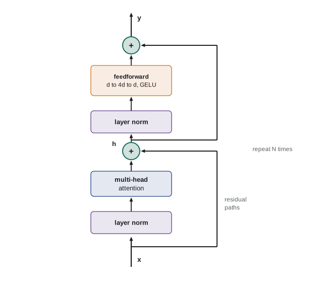
The feedforward layers hold about two thirds of a standard transformer's parameters, and evidence suggests they store much of a model's factual knowledge, acting like key-value memories (Mor Geva and colleagues, 2021). Mixture-of-experts layers replace the single feedforward network with many expert networks and a router that sends each token to a few of them, increasing parameters without increasing computation per token; AI-480 covers how they are distributed across hardware.

Costs: quadratic attention and the KV cache

For a sequence of length T and width d, the projections and feedforward layers cost on the order of \(Td^2\) operations per layer, while the attention scores cost on the order of \(T^2 d\) and need a \(T \times T\) matrix per head. For short sequences the \(d^2\) terms dominate; beyond T of a few thousand, attention's quadratic cost dominates and its memory becomes the bottleneck. FlashAttention (Tri Dao and colleagues, 2022) computes exact attention in blocks that fit in fast on-chip memory without ever writing the full score matrix to slow memory, making long contexts practical. Approximate methods (sparse, low-rank and linear attention) reduce the asymptotic cost with some loss of quality; the state space models of lesson 7 take a different route.

Generation adds a different cost. A decoder produces one token at a time, and each new token's query must attend to the keys and values of all previous tokens. Recomputing them at every step would be wasteful, so they are stored in a key-value cache and only the new token's keys and values are computed. The cache grows linearly with context length and with the number of layers and key-value heads, and for long contexts and many simultaneous users it, rather than the weights, often limits how many requests a server can handle. Grouped-query attention, quantized caches and paged memory management all target it; AI-410 covers inference serving.

# Parameter and compute accounting for a GPT-2-small-sized decoder (12 layers, d = 768, vocabulary 50,257).
L, d, V, T, heads = 12, 768, 50257, 1024, 12
attn = 4 * d * d + 4 * d                  # Wq, Wk, Wv, Wo and their biases
mlp = 2 * d * (4 * d) + 4 * d + d         # d -> 4d -> d with biases
norms = 2 * 2 * d                         # two layer norms (scale and shift) per block
block = attn + mlp + norms
emb = V * d + T * d                       # token embeddings (shared with the output layer) + learned positions
total = L * block + emb + 2 * d           # plus the final layer norm
print(f"per block: attention {attn:,}, MLP {mlp:,}, norms {norms:,} -> {block:,}")
print(f"embeddings {emb:,};  total {total:,} parameters (about {total / 1e6:.0f} M)")
N = L * block                             # non-embedding parameters
print(f"training compute per token is about 6N = {6 * N / 1e9:.2f} GFLOPs, plus attention scores 6*L*T*d = {6 * L * T * d / 1e9:.2f} GFLOPs")
kv = 2 * L * T * d * 2                    # keys and values, all layers, 16-bit numbers (2 bytes)
print(f"KV cache for one 1,024-token sequence in 16-bit: {kv / 2 ** 20:.0f} MiB")
print(f"attention score matrix per head per layer at T = 1,024: {T * T:,} entries; at T = 32,768: {32768 ** 2:,}")

per block: attention 2,362,368, MLP 4,722,432, norms 3,072 -> 7,087,872
embeddings 39,383,808;  total 124,439,808 parameters (about 124 M)
training compute per token is about 6N = 0.51 GFLOPs, plus attention scores 6*L*T*d = 0.06 GFLOPs
KV cache for one 1,024-token sequence in 16-bit: 36 MiB
attention score matrix per head per layer at T = 1,024: 1,048,576 entries; at T = 32,768: 1,073,741,824

The count reproduces GPT-2 small's published 124 million parameters, of which about 39 million are the embeddings (the token embedding matrix is shared with the output layer). The rule of thumb that a forward and backward pass costs about 6N floating-point operations per token for N non-embedding parameters (2N forward, 4N backward) is due to Jared Kaplan and colleagues (2020) and underlies the compute estimates of lesson 9.

Why transformers won

Transformers make few assumptions about their input beyond what positional information supplies, which is a weakness on small data, where convolution's built-in locality helps, and a strength at scale, where the data can teach the model which interactions matter. They parallelize fully across positions during training, which suits GPUs, and their performance has kept improving predictably as data, parameters and compute grow (lesson 9). The same architecture, with only the input embedding changed, processes text tokens, image patches, audio frames, actions and amino acids, which made multimodal models straightforward. Whether attention will remain dominant as context lengths grow is an open question, but as of 2026 the transformer remains the default architecture for large models.

Worked examples