Initialization, normalization and residual networks

Lesson 1 showed that gradients passing backward through many layers are multiplied by many factors, and lesson 3 showed that optimizers struggle when curvature differs wildly between directions. This lesson covers the three techniques that, between 2010 and 2016, turned networks of a hundred or more layers from impossible to routine. Careful initialization keeps the size of signals roughly constant from layer to layer at the start of training. Normalization layers keep them under control throughout training. Residual connections give gradients a direct path through the network. Together they are present in essentially every modern architecture, from ResNets to transformers.

Signal propagation and initialization

Consider a layer \(\mathbf{z} = W\mathbf{h}\) with \(n_{\text{in}}\) inputs, weights drawn independently with mean zero and variance \(\sigma_w^2\), and inputs with mean zero and variance \(v\). Each output is a sum of \(n_{\text{in}}\) independent terms, so its variance is \(n_{\text{in}}\sigma_w^2 v\). If \(n_{\text{in}}\sigma_w^2 > 1\), variance grows geometrically with depth and activations explode; if it is less than 1, they shrink geometrically and vanish. The same argument applied to the backward pass, where gradients are multiplied by \(W^{\top}\), gives a factor \(n_{\text{out}}\sigma_w^2\) per layer. Initialization is the choice of \(\sigma_w\) that keeps these factors near 1.

For activations that are roughly linear near zero, such as tanh, Xavier Glorot and Yoshua Bengio (2010) proposed

which compromises between the forward condition \(n_{\text{in}}\sigma_w^2 = 1\) and the backward condition \(n_{\text{out}}\sigma_w^2 = 1\). ReLU zeroes half of its inputs on average, which halves the second moment of its outputs, so Kaiming He, Xiangyu Zhang, Shaoqing Ren and Jian Sun (2015) doubled the variance to \(2/n_{\text{in}}\). Uniform versions with the same variance are also common. Biases are usually initialized to zero. The output layer is sometimes initialized smaller, or to zero, so that the network starts close to predicting the prior.

# How initialization scale controls signal size through 50 layers of width 256.
import numpy as np
rng = np.random.default_rng(466)
width, depth = 256, 50
x = rng.normal(size=(500, width))
schemes = {
    "N(0, 0.01^2), tanh":      (lambda m: rng.normal(0, 0.01, (m, m)), np.tanh),
    "N(0, 1), tanh":           (lambda m: rng.normal(0, 1.0, (m, m)), np.tanh),
    "Xavier, tanh":            (lambda m: rng.normal(0, np.sqrt(1 / m), (m, m)), np.tanh),
    "Xavier, ReLU":            (lambda m: rng.normal(0, np.sqrt(1 / m), (m, m)), lambda z: np.maximum(0, z)),
    "He, ReLU":                (lambda m: rng.normal(0, np.sqrt(2 / m), (m, m)), lambda z: np.maximum(0, z)),
}
for name, (make, act) in schemes.items():
    h = x; stds = []
    for layer in range(depth):
        h = act(h @ make(width))
        stds.append(h.std())
    print(f"{name:20} activation std after layers 1, 10, 50: {stds[0]:9.3e} {stds[9]:9.3e} {stds[49]:9.3e}")

N(0, 0.01^2), tanh   activation std after layers 1, 10, 50: 1.558e-01 1.065e-08 1.702e-40
N(0, 1), tanh        activation std after layers 1, 10, 50: 9.750e-01 9.743e-01 9.740e-01
Xavier, tanh         activation std after layers 1, 10, 50: 6.280e-01 2.243e-01 1.124e-01
Xavier, ReLU         activation std after layers 1, 10, 50: 5.859e-01 2.440e-02 3.578e-08
He, ReLU             activation std after layers 1, 10, 50: 8.286e-01 7.694e-01 1.189e+00

The output shows each failure. With weights of standard deviation 0.01, each tanh layer multiplies the scale by about \(\sqrt{256} \times 0.01 = 0.16\), and after 50 layers the activations are around \(10^{-40}\): numerically zero. With standard normal weights, pre-activations are huge and every tanh unit saturates at \(\pm 1\), so the forward signal survives but the gradients through those saturated units vanish. Xavier keeps tanh activations at a usable scale, decaying only slowly because tanh's slope is slightly below 1 away from zero. For ReLU, Xavier is too small by a factor of \(\sqrt{2}\) per layer, so activations shrink by about \(2^{-25}\) over 50 layers, while He initialization holds them steady. Choosing the initialization to match the activation is the simplest fix for deep training failures.

Mean-field analyses by Ben Poole, Samuel Schoenholz and colleagues (2016, 2017) refined this picture: for very deep networks to train, initialization must put the network at the edge of chaos, where correlations between inputs neither collapse nor decorrelate with depth, and dynamical isometry (all singular values of the input-output Jacobian near 1) helps further. With orthogonal initialization and careful scaling, Lechao Xiao and colleagues (2018) trained plain convolutional networks of 10,000 layers without normalization or residual connections. In practice, normalization and residuals make training far less sensitive to these details.

Batch normalization

Batch normalization, introduced by Sergey Ioffe and Christian Szegedy (2015), normalizes each feature using the statistics of the current mini-batch. For a feature with batch values \(x_1, \dots, x_B\),

where \(\mu_{\mathcal{B}}\) and \(\sigma_{\mathcal{B}}^2\) are the batch mean and variance and the learned scale \(\gamma\) and shift \(\beta\) let the network undo the normalization where that helps. Placed after a linear or convolutional layer and before the activation, it keeps pre-activations centered with unit variance regardless of how earlier weights change. Networks with batch normalization tolerate learning rates many times larger, are much less sensitive to initialization, and train in far fewer steps. It made networks such as Inception and ResNet practical.

The original explanation, reducing internal covariate shift (the change in each layer's input distribution as earlier layers update), has been questioned. Shibani Santurkar and colleagues (2018) showed that injecting distribution shift after batch normalization barely hurts training, and argued that batch normalization works mainly by making the loss landscape smoother, so that gradients are more predictive and larger steps are safe. It also has a regularizing effect, because each example's output depends on the other examples in its batch, a form of noise.

Batch normalization has three practical complications. At inference time there may be no batch, so running averages of the mean and variance collected during training are used instead, and forgetting to switch a framework into evaluation mode is a common bug. It behaves poorly with small batches, where batch statistics are noisy. And it couples examples within a batch, which complicates distributed training and sequence models. The backward pass is a good exercise in the chain rule because the mean and variance depend on every example; the next program derives and checks it.

# Batch normalization: forward pass, hand-derived backward pass, and a gradient check.
import numpy as np
rng = np.random.default_rng(466)
X = rng.normal(3.0, 5.0, size=(8, 4))          # a batch of 8 examples, 4 features, far from zero mean
gamma, beta, eps = rng.normal(1, 0.1, 4), rng.normal(0, 0.1, 4), 1e-5
def bn_forward(X):
    mu = X.mean(0); var = X.var(0)
    xhat = (X - mu) / np.sqrt(var + eps)
    return gamma * xhat + beta, (xhat, var)
def bn_backward(dout, cache):
    xhat, var = cache; n = len(xhat)
    dgamma = (dout * xhat).sum(0); dbeta = dout.sum(0)
    dxhat = dout * gamma                         # compact form of the chain rule through mean and variance
    dX = (n * dxhat - dxhat.sum(0) - xhat * (dxhat * xhat).sum(0)) / (n * np.sqrt(var + eps))
    return dX, dgamma, dbeta
Y, cache = bn_forward(X)
print("output means:", np.round(Y.mean(0), 3) + 0.0, " output stds:", np.round(Y.std(0), 3))
W = rng.normal(size=Y.shape)                    # loss = sum(W * Y), so dL/dY = W
dX, dg, db = bn_backward(W, cache)
num = np.zeros_like(X); h = 1e-6
for idx in np.ndindex(X.shape):
    Xp = X.copy(); Xp[idx] += h; Xm = X.copy(); Xm[idx] -= h
    num[idx] = (np.sum(W * bn_forward(Xp)[0]) - np.sum(W * bn_forward(Xm)[0])) / (2 * h)
print(f"relative error of dX: {np.linalg.norm(num - dX) / np.linalg.norm(num + dX):.2e}")
print("each column of dX sums to zero:", np.allclose(dX.sum(0), 0))

output means: [ 0.163 -0.117  0.035 -0.025]  output stds: [0.928 1.008 0.847 1.07 ]
relative error of dX: 1.23e-09
each column of dX sums to zero: True

The columns of the input gradient sum to zero: shifting every example's value of a feature by the same amount changes nothing after normalization, so the gradient can have no component in that direction.

Layer normalization and RMSNorm

Layer normalization (Jimmy Ba, Jamie Kiros and Geoffrey Hinton, 2016) normalizes across the features of each example separately, instead of across the batch for each feature. It needs no batch statistics, behaves identically in training and inference, and works for sequences of any length, so it became the normalization of choice for recurrent networks and transformers. RMSNorm (Biao Zhang and Rico Sennrich, 2019) drops the mean subtraction and divides by the root mean square, \(y = \gamma \odot \mathbf{x}/\sqrt{\frac{1}{d}\sum_j x_j^2 + \epsilon}\), which is slightly cheaper and performs as well; it is used in most recent large language models, including the Llama family. Group normalization (Yuxin Wu and Kaiming He, 2018) normalizes groups of channels within each example and suits vision models trained with small batches.

# Batch norm, layer norm and RMSNorm normalize over different axes.
import numpy as np
rng = np.random.default_rng(466)
H = rng.normal(2.0, 3.0, size=(4, 6))          # 4 examples (rows) x 6 features (columns)
bn = (H - H.mean(0)) / H.std(0)                  # per feature, across the batch
ln = (H - H.mean(1, keepdims=True)) / H.std(1, keepdims=True)   # per example, across features
rms = H / np.sqrt((H ** 2).mean(1, keepdims=True))              # per example, no centring
for name, Z in (("batch norm", bn), ("layer norm", ln), ("RMSNorm", rms)):
    print(f"{name:10} column means {np.round(Z.mean(0), 2) + 0.0}")
    print(f"{'':10} row means    {np.round(Z.mean(1), 2) + 0.0}   row RMS {np.round(np.sqrt((Z ** 2).mean(1)), 2)}")

batch norm column means [0. 0. 0. 0. 0. 0.]
           row means    [ 0.25  0.28 -0.25 -0.28]   row RMS [1.22 0.85 0.81 1.07]
layer norm column means [-0.23 -0.79 -0.06  0.55 -0.08  0.61]
           row means    [0. 0. 0. 0.]   row RMS [1. 1. 1. 1.]
RMSNorm    column means [0.52 0.19 0.77 1.03 0.46 1.06]
           row means    [0.79 0.8  0.8  0.29]   row RMS [1. 1. 1. 1.]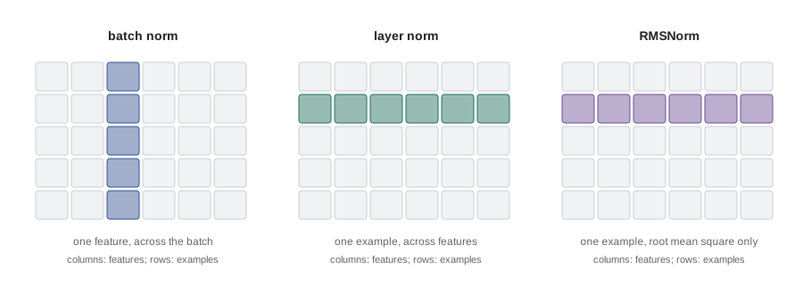

Residual connections

Even with good initialization and batch normalization, plain networks get worse as they get deeper beyond about 20 to 30 layers, and not because of overfitting: the training error itself rises. Kaiming He, Xiangyu Zhang, Shaoqing Ren and Jian Sun (2016) called this the degradation problem and noted that it is strange, since a deeper network could in principle copy a shallower one and set the extra layers to the identity. Their fix, the residual network or ResNet, makes the identity the default. Each block computes

so the block only has to learn a correction F to its input. If the best thing a block can do is nothing, it can drive F toward zero, which is easy. ResNets with 152 layers won the 2015 ImageNet competition with a top-5 error of 3.57 percent, and versions with more than 1,000 layers were trained on smaller data sets.

The gradient explains why residuals work. Differentiating the block gives \(\partial \mathbf{h}_{\ell+1}/\partial \mathbf{h}_\ell = I + \partial F/\partial \mathbf{h}_\ell\), so the gradient reaching layer \(\ell\) from the loss is the gradient at the top plus terms passing through the residual branches. The identity terms provide a direct path from the loss to every layer, and the gradient cannot vanish merely because of depth. Andreas Veit, Michael Wilber and Serge Belongie (2016) offered a complementary view: unrolling the sum shows that a residual network behaves like an ensemble of many paths of different lengths, most of them short.

# Gradient flow through 60 layers with and without residual connections (no normalization).
import numpy as np
rng = np.random.default_rng(466)
width, depth = 64, 60
x = rng.normal(size=(32, width))
def grad_norms(residual, scale):
    Ws = [rng.normal(0, scale / np.sqrt(width), (width, width)) for _ in range(depth)]
    hs = [x]; zs = []
    for W in Ws:                                 # forward: h <- h + relu(h W)  or  h <- relu(h W)
        z = hs[-1] @ W; zs.append(z)
        f = np.maximum(0, z)
        hs.append(hs[-1] + f if residual else f)
    g = np.ones_like(hs[-1]) / hs[-1].size       # gradient of mean(h_L)
    norms = []
    for W, z in zip(reversed(Ws), reversed(zs)): # backward
        gf = (g * (z > 0)) @ W.T
        g = g + gf if residual else gf
        norms.append(np.linalg.norm(g))
    return norms[::-1]
plain = grad_norms(False, np.sqrt(2) * 0.8)     # slightly below He scale
res = grad_norms(True, 0.1)                      # residual branches start small
for k in (0, 19, 39, 59):
    print(f"layer {k + 1:2}: gradient norm  plain {plain[k]:9.3e}   residual {res[k]:9.3e}")

layer  1: gradient norm  plain 3.909e-07   residual 1.711e-01
layer 20: gradient norm  plain 1.284e-05   residual 1.042e-01
layer 40: gradient norm  plain 6.875e-04   residual 4.910e-02
layer 60: gradient norm  plain 1.996e-02   residual 2.285e-02

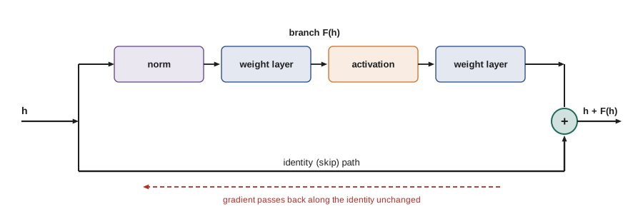
In the plain network the gradient shrinks by a roughly constant factor per layer, so at layer 1 it is about 50,000 times smaller than at layer 60, and the early layers barely learn. In the residual network the gradient at layer 1 is within a factor of about eight of the gradient at layer 60, and it grows rather than shrinks going down, because each block adds its branch contribution to the identity path. With unscaled branches that growth would itself become a problem, which is why branch scale matters. Two design details make residual networks robust in practice. First, the residual branch is often initialized so that F starts near zero: zero-initializing the last scale parameter in each block (Priya Goyal and colleagues, 2017) or scaling branch weights down with depth (as in GPT-2, which scales by \(1/\sqrt{N}\) for N residual layers). Second, where the normalization goes matters. The original ResNet and transformer placed it after the addition (post-norm). Pre-norm, which normalizes the input to the branch, \(\mathbf{h} + F(\mathrm{Norm}(\mathbf{h}))\), keeps the identity path completely clean, trains stably without careful warmup, and is the standard in large transformers (Ruibin Xiong and colleagues, 2020).

Putting the pieces together

A modern deep block combines all three ideas: a normalization layer, one or two weight layers with a nonlinearity, and a residual connection, with weights initialized by a He- or Xavier-style rule and residual branches scaled down. The transformer block of lesson 8 is exactly this pattern twice over, once around attention and once around a feedforward network. When a deep model fails to train, the checklist starts here: are activations and gradients of reasonable size at every layer at initialization, is every block residual, is normalization present and in evaluation mode at test time, and is the learning rate warmed up? Lesson 11 turns this into a debugging procedure.

Normalization-free alternatives exist and show that the pieces are partly interchangeable. Fixup initialization (Hongyi Zhang and colleagues, 2019) trains deep ResNets without normalization by rescaling residual branches at initialization, and NFNets (Andrew Brock and colleagues, 2021) reached strong ImageNet accuracy without batch normalization by combining scaled residual branches with adaptive gradient clipping. The common thread is controlling the size of signals and gradients at every depth.

Worked examples