Convolutional networks

A fully connected layer treats its input as an unordered list of numbers. For an image, that throws away the most important fact about the data: pixels near each other are related, and the same pattern means the same thing wherever it appears. Convolutional neural networks (CNNs) build these two facts into the architecture through local connectivity and weight sharing. The result needs far fewer parameters, learns from far less data, and responds predictably when an object moves. This lesson develops convolution precisely, including the arithmetic of sizes, strides, padding and receptive fields that every practitioner must be able to do in their head, then follows the architectural ideas from LeNet to ResNet and efficient modern designs. AI-350 applies CNNs to detection, segmentation and other vision tasks; this lesson is about how they work.

From dense layers to convolutions

A 224 × 224 color image has 150,528 input values. A dense layer from it to even 1,000 hidden units needs 150 million weights, almost all of them connecting pixels to features in faraway parts of the image that they have nothing to do with. Two assumptions cut this down. Locality: a feature at a position depends only on a small neighborhood around it, say 3 × 3 or 5 × 5 pixels. Stationarity: the same feature detector is useful everywhere, so the weights for detecting a vertical edge at the top left can be reused at the bottom right. Imposing both on a dense layer turns it into a convolution: a small kernel of weights slides over the image, computing a weighted sum at every position.

Formally, for a single-channel input x and kernel k of size \(K \times K\), the output is

Strictly this is cross-correlation; true convolution flips the kernel. Since the kernel is learned, the flip makes no difference, and every deep learning library computes cross-correlation while calling it convolution. With C input channels and D output channels, the kernel becomes a tensor of shape \(D \times C \times K \times K\): each output channel sums a K × K filter over every input channel. Each output channel is called a feature map.

# 2-D convolution (strictly, cross-correlation, as in every deep learning library) written from scratch.
import numpy as np
def conv2d(x, k, stride=1, pad=0):
    x = np.pad(x, pad)
    kh, kw = k.shape
    oh = (x.shape[0] - kh) // stride + 1; ow = (x.shape[1] - kw) // stride + 1
    out = np.zeros((oh, ow))
    for i in range(oh):
        for j in range(ow):
            patch = x[i * stride:i * stride + kh, j * stride:j * stride + kw]
            out[i, j] = np.sum(patch * k)           # same kernel weights at every position
    return out
img = np.zeros((7, 7)); img[1:6, 2:5] = 1.0         # a bright 5 x 3 rectangle on a dark background
sobel_x = np.array([[-1, 0, 1], [-2, 0, 2], [-1, 0, 1]], dtype=float)   # responds to left-right edges
print("image:\n", img.astype(int))
print("vertical-edge response (no padding, 5 x 5):\n", conv2d(img, sobel_x).astype(int))
shifted = np.roll(img, 1, axis=1)                  # move the rectangle one pixel right
a, b = conv2d(img, sobel_x, pad=1), conv2d(shifted, sobel_x, pad=1)
print("translation equivariance: response to shifted image equals shifted response:",
      np.allclose(b[:, 1:], a[:, :-1]))
print("output size with stride 2 and padding 1:", conv2d(img, sobel_x, stride=2, pad=1).shape)

image:
 [[0 0 0 0 0 0 0]
 [0 0 1 1 1 0 0]
 [0 0 1 1 1 0 0]
 [0 0 1 1 1 0 0]
 [0 0 1 1 1 0 0]
 [0 0 1 1 1 0 0]
 [0 0 0 0 0 0 0]]
vertical-edge response (no padding, 5 x 5):
 [[ 3  3  0 -3 -3]
 [ 4  4  0 -4 -4]
 [ 4  4  0 -4 -4]
 [ 4  4  0 -4 -4]
 [ 3  3  0 -3 -3]]
translation equivariance: response to shifted image equals shifted response: True
output size with stride 2 and padding 1: (4, 4)

The edge detector responds positively at the rectangle's left edge (dark to bright, moving right) and negatively at its right edge, and is zero in flat regions. In a trained CNN, nobody writes such kernels: the first layer's filters are learned, and they reliably come out looking like oriented edge and color detectors, much like the receptive fields David Hubel and Torsten Wiesel found in the cat's visual cortex in 1959, the work that inspired Kunihiko Fukushima's neocognitron (1980) and, through it, CNNs.

Equivariance and invariance

Weight sharing gives convolution a precise property: translation equivariance. If the input shifts by some amount, the output feature map shifts by the same amount, as the program confirms. This is exactly right for detecting features: a cat's ear is an ear wherever it is. For classifying the whole image we want invariance, an output that does not change when the object moves, and networks obtain approximate invariance by pooling and by the large receptive fields of deep layers. The equivariance is only approximate in practice, because strided layers and pooling break it for shifts that are not multiples of the stride; Richard Zhang (2019) showed that small shifts can noticeably change the predictions of standard CNNs and that blurring before downsampling (anti-aliasing) restores much of the lost consistency.

Size arithmetic: padding, stride and dilation

For input size n, kernel size k, padding p and stride s, the output size along each dimension is

Without padding, each 3 × 3 layer shrinks the map by 2 and the borders are seen by fewer kernel positions. Same padding, p = (k − 1)/2 for odd k, keeps the size unchanged at stride 1. A stride of 2 halves the resolution, which is the usual way of downsampling inside a network. Dilated convolutions insert gaps between kernel taps, so a 3 × 3 kernel with dilation 2 covers a 5 × 5 area with nine weights; they enlarge the receptive field without losing resolution and are used in segmentation and audio models such as WaveNet. Transposed convolutions run the arithmetic in reverse to upsample, as in decoder networks.

Receptive fields

The receptive field of a unit is the region of the input that can affect it. A 3 × 3 convolution has a receptive field of 3; stacking a second 3 × 3 layer gives 5, a third gives 7. Strides multiply the effect of later layers: after a stride-2 layer, each step in the feature map corresponds to two input pixels, so the next 3 × 3 layer adds 4 to the receptive field instead of 2. The recurrence is \(r_{\ell} = r_{\ell-1} + (k_\ell - 1)\,j_{\ell-1}\) and \(j_\ell = j_{\ell-1}s_\ell\), where j is the jump, the input distance between neighboring units. Deep layers therefore see large regions, which is how a network with only 3 × 3 kernels can recognize whole objects. The theoretical receptive field overstates the effective one: Wenjie Luo and colleagues (2016) showed that the influence of input pixels falls off roughly like a Gaussian from the center, so the region that matters in practice is much smaller.

# Output sizes, receptive fields and parameter counts for a small convolutional stack on 224 x 224 x 3 input.
layers = [  # (name, kernel, stride, padding, out_channels); pooling has out_channels None
    ("conv 7x7/2", 7, 2, 3, 64), ("maxpool 3x3/2", 3, 2, 1, None),
    ("conv 3x3", 3, 1, 1, 64), ("conv 3x3", 3, 1, 1, 64),
    ("conv 3x3/2", 3, 2, 1, 128), ("conv 3x3", 3, 1, 1, 128),
    ("conv 3x3/2", 3, 2, 1, 256), ("conv 3x3", 3, 1, 1, 256),
]
size, ch, rf, jump, total = 224, 3, 1, 1, 0
print(f"{'layer':14} {'output':>14} {'receptive field':>16} {'parameters':>11}")
for name, k, s, p, out in layers:
    size = (size + 2 * p - k) // s + 1
    rf = rf + (k - 1) * jump                       # each layer widens the field by (k-1) input jumps
    jump *= s                                      # distance between adjacent outputs, in input pixels
    params = 0 if out is None else k * k * ch * out + out
    if out is not None:
        ch = out
    total += params
    print(f"{name:14} {f'{size}x{size}x{ch}':>14} {rf:>16} {params:>11,}")
print(f"total parameters {total:,}")
dense = 224 * 224 * 3 * 64
print(f"a dense layer from the raw image to just 64 units would need {dense:,} weights")

layer                  output  receptive field  parameters
conv 7x7/2         112x112x64                7       9,472
maxpool 3x3/2        56x56x64               11           0
conv 3x3             56x56x64               19      36,928
conv 3x3             56x56x64               27      36,928
conv 3x3/2          28x28x128               35      73,856
conv 3x3            28x28x128               51     147,584
conv 3x3/2          14x14x256               67     295,168
conv 3x3            14x14x256               99     590,080
total parameters 1,190,016
a dense layer from the raw image to just 64 units would need 9,633,792 weights

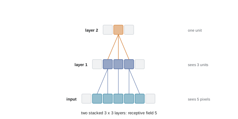
Stacking small kernels is better than using one large one. Two 3 × 3 layers have the receptive field of one 5 × 5 layer with 18 rather than 25 weights per channel pair, and three 3 × 3 layers match a 7 × 7 with 27 rather than 49, while adding nonlinearities between them. This observation drove the VGG design.

Pooling

Pooling layers downsample by summarizing small windows. Max pooling keeps the largest value in each window, typically 2 × 2 with stride 2, signaling whether a feature was present anywhere in the window and giving a little invariance to small shifts. Average pooling keeps the mean. Global average pooling, introduced in the Network in Network architecture (Min Lin and colleagues, 2014), averages each feature map over all positions to a single number, producing a fixed-length vector regardless of input size, and replaced the huge fully connected layers at the end of earlier networks. Many modern designs use strided convolutions instead of pooling for downsampling, letting the network learn how to summarize.

# Pooling gives a little invariance to small shifts; global average pooling summarizes each channel.
import numpy as np
fmap = np.array([[0, 0, 0, 0], [0, 9, 0, 0], [0, 0, 0, 0], [0, 0, 0, 0]], dtype=float)
def maxpool2(x):
    return x.reshape(x.shape[0] // 2, 2, x.shape[1] // 2, 2).max(axis=(1, 3))
print("feature map peak at (1, 1); 2x2 max pool:\n", maxpool2(fmap))
print("peak moved to (0, 0), same pool output:", np.array_equal(maxpool2(np.roll(fmap, (-1, -1), (0, 1))), maxpool2(fmap)))
print("peak moved to (1, 2), crosses a pooling boundary:\n", maxpool2(np.roll(fmap, 1, 1)))
rng = np.random.default_rng(466)
feats = rng.normal(size=(512, 7, 7))       # 512 channels of 7x7 at the end of a network
print("global average pooling turns", feats.shape, "into a vector of", feats.mean(axis=(1, 2)).shape)

feature map peak at (1, 1); 2x2 max pool:
 [[9. 0.]
 [0. 0.]]
peak moved to (0, 0), same pool output: True
peak moved to (1, 2), crosses a pooling boundary:
 [[0. 9.]
 [0. 0.]]
global average pooling turns (512, 7, 7) into a vector of (512,)

A short history of architectures

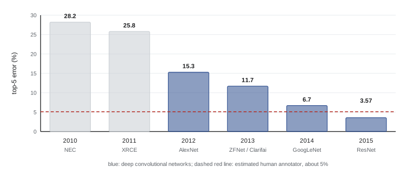
LeNet-5 (Yann LeCun and colleagues, 1998) read handwritten digits and check amounts with two convolutional layers, subsampling and three dense layers, about 60,000 parameters in all. AlexNet (Alex Krizhevsky, Ilya Sutskever and Geoffrey Hinton, 2012), trained at the University of Toronto on two consumer graphics cards, won the ImageNet Large Scale Visual Recognition Challenge with a top-5 error of 15.3 percent against 26.2 percent for the runner-up, and began the deep learning era. Its ingredients, ReLU, dropout, data augmentation and GPU training, were as important as its depth. VGG (Karen Simonyan and Andrew Zisserman, 2014) showed that a simple stack of 3 × 3 convolutions, 16 to 19 layers deep, did better still. GoogLeNet or Inception (Christian Szegedy and colleagues, 2014) ran convolutions of several sizes in parallel and used 1 × 1 convolutions to cut channels cheaply. ResNet (lesson 4) made 152 layers trainable and won in 2015 with 3.57 percent top-5 error, below the roughly 5 percent estimated for a trained human annotator on that benchmark.

A 1 × 1 convolution deserves a note: it applies the same small dense layer to the channel vector at every position, mixing channels without looking at neighbors. It is the standard way to change the number of channels, and ResNet's bottleneck blocks use a 1 × 1 layer to reduce channels, a 3 × 3 layer at the reduced width, and a second 1 × 1 layer to restore them.

Efficient convolutions

For phones and embedded devices, cost matters as much as accuracy. A depthwise separable convolution factors a standard convolution into a depthwise step, one K × K filter per input channel with no mixing, followed by a pointwise 1 × 1 convolution that mixes channels. MobileNet (Andrew Howard and colleagues, 2017) built on this; for 3 × 3 kernels it cuts parameters and computation by a factor of about 8 to 9 with a modest loss of accuracy. EfficientNet (Mingxing Tan and Quoc Le, 2019) scaled depth, width and input resolution together by a compound rule found by search, and ConvNeXt (Zhuang Liu and colleagues, 2022) showed that a CNN modernized with ideas borrowed from transformers (larger depthwise kernels, layer normalization, GELU, fewer activations) matches vision transformers at similar cost. Vision transformers, which apply the attention of lesson 8 to image patches, are covered in AI-350; on very large data they have overtaken CNNs for many tasks, but CNNs remain strong, efficient and widely deployed, especially where data or computation are limited.

# Standard versus depthwise separable convolution: parameters and multiply-adds for one layer.
H = W = 56; cin, cout, k = 128, 128, 3
std_params = k * k * cin * cout
dw_params = k * k * cin                    # one k x k filter per input channel
pw_params = cin * cout                     # then a 1 x 1 convolution mixes channels
std_macs = std_params * H * W
sep_macs = (dw_params + pw_params) * H * W
print(f"standard 3x3:        {std_params:>9,} parameters, {std_macs / 1e6:7.1f} M multiply-adds")
print(f"depthwise separable: {dw_params + pw_params:>9,} parameters, {sep_macs / 1e6:7.1f} M multiply-adds")
print(f"ratio: {std_params / (dw_params + pw_params):.1f}x fewer (theory: 1 / (1/cout + 1/k^2) = {1 / (1 / cout + 1 / k ** 2):.1f})")

standard 3x3:          147,456 parameters,   462.4 M multiply-adds
depthwise separable:    17,536 parameters,    55.0 M multiply-adds
ratio: 8.4x fewer (theory: 1 / (1/cout + 1/k^2) = 8.4)

Beyond images

Convolution applies wherever data lie on a grid with local, repeated structure. One-dimensional convolutions process audio waveforms, sensor time series and, in some models, text; dilated causal 1-D convolutions let WaveNet (Aäron van den Oord and colleagues, 2016) model raw audio with receptive fields of thousands of samples. Three-dimensional convolutions process video and volumetric medical scans. Graph neural networks (lesson 9) generalize the idea of a shared local operation to irregular neighborhoods. The design principle carries over: build the symmetries of the data into the architecture, and the network does not have to learn them from examples.

Worked examples