Backpropagation and automatic differentiation

Every network in this course is trained by gradient descent, which needs the gradient of the loss with respect to every parameter. Lesson 1 wrote those gradients by hand, which is tedious for two layers and impossible for a hundred. This lesson explains how gradients are computed automatically and efficiently. It frames a network as a computational graph, derives backpropagation as reverse-mode automatic differentiation on that graph, implements a working autodiff engine in about forty lines, and shows how to verify any gradient with finite differences. It also covers the loss functions and output layers that sit at the top of the graph, and the numerical tricks needed to compute them safely.

AI-210 and AI-310 introduce automatic differentiation from the mathematical and optimization sides. Here the emphasis is on the algorithm as a computing scientist would implement it, its cost, and how it is used and debugged in deep learning systems.

Computational graphs

Any computation built from elementary operations can be drawn as a directed acyclic graph. Leaves are inputs and parameters; internal nodes are operations such as addition, multiplication, matrix product, tanh or exp; edges carry values from operands to results. The loss is a single node at the top. For \(f(x, y) = \tanh(xy + x)\,e^{y}\), the graph has a multiplication node for \(xy\), an addition node, a tanh node, an exp node and a final multiplication. The input x feeds two nodes, a detail that matters for the gradient.

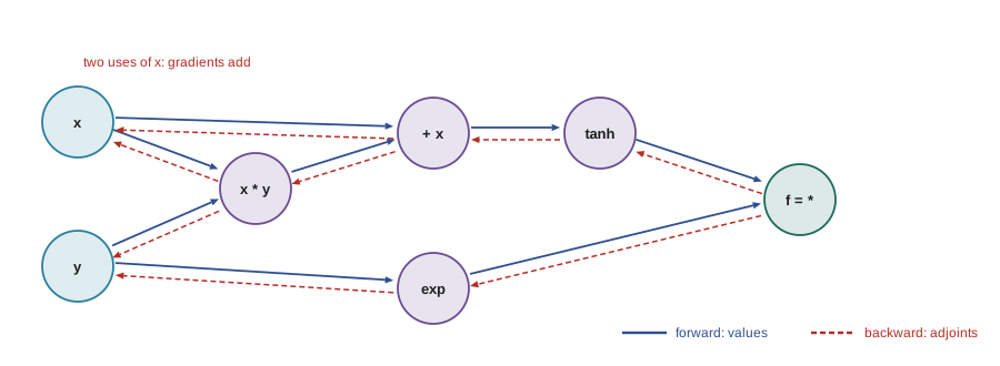
The chain rule says how to differentiate through the graph. If a node v feeds several nodes \(u_1, \dots, u_k\), each of which eventually affects the output f, then

The quantity \(\bar{v} = \partial f / \partial v\) is called the adjoint of v. The rule says that a node's adjoint is the sum, over the nodes it feeds, of their adjoints times the local derivative of each operation with respect to v. Each local derivative is simple: for \(u = a + b\) it is 1 for both operands; for \(u = ab\) it is b for a and a for b; for \(u = \tanh(a)\) it is \(1 - u^2\); for \(u = e^{a}\) it is u.

Reverse mode: backpropagation

Reverse-mode automatic differentiation computes all adjoints in two sweeps. The forward sweep evaluates the graph in topological order and stores each node's value. The backward sweep sets the output's adjoint to 1 and visits nodes in reverse topological order; at each node it adds the node's adjoint, times the local derivative, into each parent's adjoint. When the sweep finishes, every leaf holds the partial derivative of f with respect to it. Backpropagation, as popularized for neural networks by David Rumelhart, Geoffrey Hinton and Ronald Williams in 1986, is exactly this algorithm applied to a network's graph. Its earlier history includes Seppo Linnainmaa's 1970 master's thesis, which described reverse-mode differentiation of general programs, and Paul Werbos's 1974 thesis, which applied it to neural networks.

The cost of the backward sweep is a small constant multiple of the cost of the forward sweep, typically two to three times, regardless of how many parameters there are. This is the cheap gradient principle, and it is what makes training networks with billions of parameters possible. The price is memory: the backward sweep needs the values computed in the forward sweep (the activations), so they must be stored, and for large models activation memory often exceeds parameter memory. Lesson 11 and AI-480 discuss gradient checkpointing, which trades extra computation for memory by recomputing some activations during the backward sweep.

The program below implements reverse mode for scalar values. Each Value object records its data, its parents and a closure that knows how to push its adjoint to its parents. Calling backward on the output builds a topological order by depth-first search and runs the closures in reverse. The sum in the chain rule appears as the += in each closure: because x is used twice, it receives two contributions that add up. Writing = instead of += is the classic bug in hand-written autodiff engines.

# A tiny reverse-mode automatic differentiation engine for scalars, in about 40 lines.
import math
class Value:
    def __init__(self, data, parents=(), op=""):
        self.data, self.grad, self._parents, self.op = data, 0.0, parents, op
        self._backward = lambda: None
    def __add__(self, other):
        other = other if isinstance(other, Value) else Value(other)
        out = Value(self.data + other.data, (self, other), "+")
        def backward():                      # d(a+b)/da = d(a+b)/db = 1
            self.grad += out.grad; other.grad += out.grad
        out._backward = backward; return out
    def __mul__(self, other):
        other = other if isinstance(other, Value) else Value(other)
        out = Value(self.data * other.data, (self, other), "*")
        def backward():                      # d(ab)/da = b, d(ab)/db = a
            self.grad += other.data * out.grad; other.grad += self.data * out.grad
        out._backward = backward; return out
    __radd__, __rmul__ = __add__, __mul__
    def tanh(self):
        t = math.tanh(self.data); out = Value(t, (self,), "tanh")
        def backward(): self.grad += (1 - t * t) * out.grad
        out._backward = backward; return out
    def exp(self):
        e = math.exp(self.data); out = Value(e, (self,), "exp")
        def backward(): self.grad += e * out.grad
        out._backward = backward; return out
    def backward(self):
        order, seen = [], set()
        def visit(v):                        # topological order of the graph
            if v not in seen:
                seen.add(v)
                for p in v._parents: visit(p)
                order.append(v)
        visit(self); self.grad = 1.0
        for v in reversed(order): v._backward()   # each node passes gradient to its parents
        return len(order)

# f(x, y) = tanh(x*y + x) * exp(y): x is used twice, so its gradients must add up
x, y = Value(0.5), Value(-1.2)
f = (x * y + x).tanh() * y.exp()
nodes = f.backward()
print(f"f = {f.data:.6f}, graph has {nodes} nodes")
print(f"autodiff:  df/dx = {x.grad:.6f}, df/dy = {y.grad:.6f}")
# check against central finite differences
def F(a, b): return math.tanh(a * b + a) * math.exp(b)
h = 1e-6
print(f"numerical: df/dx = {(F(0.5 + h, -1.2) - F(0.5 - h, -1.2)) / (2 * h):.6f}, "
      f"df/dy = {(F(0.5, -1.2 + h) - F(0.5, -1.2 - h)) / (2 * h):.6f}")

f = -0.030019, graph has 7 nodes
autodiff:  df/dx = -0.059640, df/dy = 0.119082
numerical: df/dx = -0.059640, df/dy = 0.119082

This is essentially the design of Andrej Karpathy's teaching library micrograd, and in miniature the design of the autograd systems in PyTorch, JAX and TensorFlow. Production systems differ in three main ways. They operate on tensors rather than scalars, so each node is a whole matrix operation with a vector-Jacobian product rule (for \(C = AB\), \(\bar{A} = \bar{C}B^{\top}\) and \(\bar{B} = A^{\top}\bar{C}\)), and the bookkeeping overhead is amortized over millions of arithmetic operations. They provide hand-optimized backward rules for hundreds of operations, fused into efficient GPU kernels. And they differ in when the graph is built: PyTorch records the graph dynamically as ordinary Python code runs (define-by-run), while JAX traces a Python function once into an intermediate representation and compiles it, which enables whole-program optimization.

Forward mode and why deep learning uses reverse mode

Automatic differentiation also has a forward mode. It carries, alongside each value, its derivative with respect to one chosen input direction, and propagates both forward through the graph. One forward-mode pass computes a Jacobian-vector product \(J\mathbf{v}\): the directional derivative of all outputs along \(\mathbf{v}\). One reverse-mode pass computes a vector-Jacobian product \(\mathbf{u}^{\top}J\): the gradient of one combination of outputs with respect to all inputs. For a function from \(\mathbb{R}^n\) to \(\mathbb{R}^m\), the full Jacobian needs n forward passes or m reverse passes.

A training loss maps millions or billions of parameters to one number, so n is enormous and m = 1. Reverse mode gets the whole gradient in one backward pass; forward mode would need one pass per parameter. Forward mode is still useful when there are few inputs and many outputs, and the two modes combine to compute Hessian-vector products cheaply (forward over reverse), which second-order optimizers and some interpretability methods use. Automatic differentiation should not be confused with symbolic differentiation, which manipulates formulas and can produce expressions that grow exponentially, or with numerical differentiation by finite differences, which is approximate and costs one or two function evaluations per input.

# Forward mode versus reverse mode: cost of a full gradient of f: R^n -> R.
# Forward mode needs one pass per input direction; reverse mode needs one backward pass.
import numpy as np
rng = np.random.default_rng(466)
n = 300
A = rng.normal(size=(n, n)) / np.sqrt(n)
def f(x): return np.sum(np.tanh(A @ x) ** 2)
x = rng.normal(size=n)

# reverse mode, written out: one forward pass and one vector-Jacobian product
u = A @ x; t = np.tanh(u)
grad_rev = A.T @ (2 * t * (1 - t ** 2))        # chain rule from the output back to x
# forward mode: Jacobian-vector product with each basis vector e_i (n passes)
grad_fwd = np.empty(n)
for i in range(n):
    du = A[:, i]                               # directional derivative of u along e_i
    grad_fwd[i] = np.sum(2 * t * (1 - t ** 2) * du)
print("max difference between modes:", float(np.max(np.abs(grad_rev - grad_fwd))))
print(f"matrix-vector products needed: reverse 2, forward {n} (one per input)")
print("for a network with a billion parameters and one loss, reverse mode is the only practical choice")

max difference between modes: 8.881784197001252e-16
matrix-vector products needed: reverse 2, forward 300 (one per input)
for a network with a billion parameters and one loss, reverse mode is the only practical choice

Loss functions and output layers

The top of the graph is the loss. Its choice follows from a probabilistic view: choose an output distribution for the target given the input, and minimize the negative log-likelihood of the training data. For regression with Gaussian noise of fixed variance, this gives the mean squared error \(\tfrac{1}{2}(\hat{y} - y)^2\) with an identity output. For binary classification with a Bernoulli output, it gives binary cross-entropy with a sigmoid output. For K classes with a categorical output, it gives cross-entropy with a softmax output,

where \(s_k\) are the scores, also called logits. In each matched pair (identity with squared error, sigmoid with binary cross-entropy, softmax with categorical cross-entropy) the gradient of the loss with respect to the scores takes the same simple form: prediction minus target. For softmax, \(\partial \mathcal{L}/\partial s_k = p_k - [k = y]\). Mismatched pairs, such as a sigmoid output trained with squared error, have gradients that vanish when the sigmoid saturates on a confidently wrong answer, which is exactly when learning is most needed.

Other losses suit other tasks. The Huber loss is quadratic near zero and linear far away, making regression robust to outliers. Label smoothing replaces the one-hot target with a mixture of the one-hot vector and a uniform distribution, for example 0.9 on the true class and the rest spread evenly, which discourages overconfident logits and often improves calibration. Focal loss down-weights easy examples and is used in detection. Contrastive losses, which compare pairs or sets of examples, appear in lesson 9.

Numerical stability: the log-sum-exp trick

Computing the softmax directly overflows as soon as any score exceeds about 88 in single precision or 709 in double precision, because \(e^{s}\) is then larger than the largest representable number. The fix uses the identity \(\log \sum_j e^{s_j} = m + \log \sum_j e^{s_j - m}\) with \(m = \max_j s_j\): after subtracting the maximum, the largest exponent is \(e^0 = 1\) and nothing overflows. Frameworks therefore provide fused functions that take logits and targets and compute cross-entropy directly (in PyTorch, cross_entropy applied to raw logits, and binary_cross_entropy_with_logits for the binary case). Applying a softmax first and then taking a logarithm separately is a common source of NaN losses.

# Why softmax and cross-entropy must be computed with the log-sum-exp trick.
import numpy as np
s = np.array([1000.0, 1001.0, 1002.0])          # large scores are common late in training
with np.errstate(over="ignore", invalid="ignore"):
    naive = np.exp(s) / np.exp(s).sum()
print("naive softmax:     ", naive)
m = s.max()
stable = np.exp(s - m) / np.exp(s - m).sum()     # same value mathematically, no overflow
print("stable softmax:    ", np.round(stable, 6))
logsumexp = m + np.log(np.exp(s - m).sum())
print("log-sum-exp:       ", round(logsumexp, 6))
print("cross-entropy if class 0 is correct:", round(logsumexp - s[0], 6))
# float32 range: exp overflows past about 88.7
print("largest x with finite exp(x) in float32:", round(float(np.log(np.finfo(np.float32).max)), 2))

naive softmax:      [nan nan nan]
stable softmax:     [0.090031 0.244728 0.665241]
log-sum-exp:        1002.407606
cross-entropy if class 0 is correct: 2.407606
largest x with finite exp(x) in float32: 88.72

Checking gradients

Hand-written backward passes and custom operations need testing, and the standard test is a gradient check: compare the analytic gradient with a central finite difference \((f(\theta + \epsilon e_i) - f(\theta - \epsilon e_i)) / 2\epsilon\) for each parameter, or for a random sample of parameters in a large model. The central difference has error of order \(\epsilon^2\), against \(\epsilon\) for the one-sided version. Compare with a relative error, \(\lVert g_{\text{num}} - g_{\text{ana}} \rVert / (\lVert g_{\text{num}} \rVert + \lVert g_{\text{ana}} \rVert)\), because absolute errors depend on scale. In double precision with \(\epsilon \approx 10^{-5}\), a correct gradient typically gives relative errors around \(10^{-7}\) or smaller; errors near \(10^{-2}\) indicate a bug.

# Gradient checking a hand-written backward pass for a small MLP with softmax cross-entropy.
import numpy as np
rng = np.random.default_rng(466)
X = rng.normal(size=(5, 4)); y = np.array([0, 2, 1, 2, 0])          # 5 examples, 3 classes
P = {"W1": rng.normal(0, 0.5, (4, 6)), "b1": np.zeros(6), "W2": rng.normal(0, 0.5, (6, 3)), "b2": np.zeros(3)}

def loss_and_grads(P):
    z1 = X @ P["W1"] + P["b1"]; h = np.tanh(z1)
    s = h @ P["W2"] + P["b2"]
    s = s - s.max(axis=1, keepdims=True)                 # log-sum-exp trick: subtract the row max
    logp = s - np.log(np.exp(s).sum(axis=1, keepdims=True))
    loss = -logp[np.arange(len(y)), y].mean()
    g = np.exp(logp); g[np.arange(len(y)), y] -= 1; g /= len(y)   # dL/ds = softmax - one-hot
    G = {"W2": h.T @ g, "b2": g.sum(0)}
    gz = (g @ P["W2"].T) * (1 - h ** 2)
    G["W1"] = X.T @ gz; G["b1"] = gz.sum(0)
    return loss, G

loss, G = loss_and_grads(P)
print(f"loss = {loss:.6f}")
eps = 1e-5
for name in P:
    num = np.zeros_like(P[name])
    for idx in np.ndindex(P[name].shape):                # perturb one parameter at a time
        old = P[name][idx]
        P[name][idx] = old + eps; lp, _ = loss_and_grads(P)
        P[name][idx] = old - eps; lm, _ = loss_and_grads(P)
        P[name][idx] = old
        num[idx] = (lp - lm) / (2 * eps)
    rel = np.linalg.norm(num - G[name]) / max(np.linalg.norm(num) + np.linalg.norm(G[name]), 1e-12)
    print(f"{name}: {P[name].size:2} entries, relative error {rel:.2e}")

loss = 0.944302
W1: 24 entries, relative error 8.80e-11
b1:  6 entries, relative error 9.99e-11
W2: 18 entries, relative error 2.76e-11
b2:  3 entries, relative error 3.70e-11

Gradient checks have traps. Use double precision, since single precision rounding swamps the difference quotient. Points where the function has a kink, such as ReLU at zero or a max, can give spurious failures if a perturbation crosses the kink. Turn off randomness such as dropout during the check, or fix its seed, so that the function is the same on every evaluation. And check on a small model and a few examples, since the check costs two loss evaluations per parameter.

Autodiff in practice

Several practical consequences follow from how autodiff works. Gradients accumulate: frameworks add into each parameter's gradient buffer, so the buffers must be zeroed before each step, and forgetting to do so silently sums gradients across steps (which is occasionally done on purpose, to simulate a larger batch, a technique called gradient accumulation). Operations that are not differentiable, such as argmax, rounding or sampling a discrete value, pass no useful gradient; workarounds include the straight-through estimator, the Gumbel-softmax relaxation and the reparameterization trick of lesson 10. Detaching a tensor from the graph (stop-gradient) blocks gradient flow on purpose, as in target networks in reinforcement learning (AI-330). In-place operations that overwrite values needed by the backward pass cause errors or wrong answers. And because the graph is built from the actual operations executed, control flow such as loops and conditionals is handled naturally: the gradient is that of the path actually taken.

Worked examples