Generative models: autoencoders, VAEs, GANs and diffusion

The models so far have been discriminative or predictive: they map inputs to labels, or predict the next token. Generative models learn the distribution of the data itself, so that they can produce new samples that look like the training data, assess how likely a given example is, or fill in missing parts. Autoregressive language models (lessons 7 and 8) are one family, factorizing the probability of a sequence token by token. This lesson covers the other main families: autoencoders and variational autoencoders, which learn a compressed latent representation; generative adversarial networks, which pit a generator against a discriminator; and diffusion models, which learn to reverse a gradual noising process and now produce most state-of-the-art images, audio and video. The aim is to understand each family's objective and its trade-offs; AI-410 and AI-350 cover large-scale image, video and multimodal generation.

What a generative model must do

Three capabilities can be asked of a generative model, and families differ in which they offer. Sampling: draw new examples from the learned distribution \(p_\theta(\mathbf{x})\). Density evaluation: compute \(p_\theta(\mathbf{x})\) or its logarithm for a given \(\mathbf{x}\), useful for anomaly detection and model comparison. Representation: map examples to a latent space in which similar examples are close and interpolation is meaningful. Autoregressive models give exact likelihoods and good samples but generate slowly, one element at a time. VAEs give a latent space and a likelihood bound. GANs give fast, sharp samples but no likelihood. Diffusion models give excellent samples and a likelihood bound, at the cost of many network evaluations per sample. Normalizing flows, which transform a simple distribution through invertible layers whose Jacobian determinants are tractable, give exact likelihoods and fast sampling but constrain the architecture; they are not covered further here.

Autoencoders

An autoencoder is a network trained to reproduce its input through a bottleneck. An encoder f maps \(\mathbf{x}\) to a code \(\mathbf{z} = f(\mathbf{x})\) of lower dimension, a decoder g maps it back, and training minimizes reconstruction error \(\lVert \mathbf{x} - g(f(\mathbf{x})) \rVert^2\). The bottleneck forces the code to keep the most important information. A linear autoencoder with squared error learns the same subspace as principal component analysis (Pierre Baldi and Kurt Hornik, 1989), which the next program confirms; deep nonlinear autoencoders learn curved low-dimensional structure that PCA cannot. Denoising autoencoders (Pascal Vincent and colleagues, 2008) corrupt the input and train the network to recover the clean version, which forces them to learn the structure of the data rather than an identity map, an idea that diffusion models take to its limit.

# A linear autoencoder with a 2-unit bottleneck, trained by gradient descent, recovers the PCA subspace.
import numpy as np
rng = np.random.default_rng(466)
Z = rng.normal(size=(500, 2)) * [3.0, 1.0]                   # data that really live near a 2-D plane
M = np.linalg.qr(rng.normal(size=(6, 2)))[0]
X = Z @ M.T + 0.1 * rng.normal(size=(500, 6)); X -= X.mean(0)
E = rng.normal(0, 0.1, (6, 2)); D = rng.normal(0, 0.1, (2, 6))   # encoder and decoder
for step in range(1, 3001):
    code = X @ E; Xh = code @ D
    G = 2 * (Xh - X) / len(X)                                   # gradient of mean squared reconstruction error
    gD = code.T @ G; gE = X.T @ (G @ D.T)
    E -= 0.01 * gE; D -= 0.01 * gD
    if step in (1, 300, 3000):
        print(f"step {step:4}: reconstruction MSE {np.mean((Xh - X) ** 2):.4f}")
_, s, Vt = np.linalg.svd(X, full_matrices=False)
pca_err = np.mean((X - X @ Vt[:2].T @ Vt[:2]) ** 2)
Qa = np.linalg.qr(D.T)[0]                                       # subspace spanned by the decoder
cos = np.linalg.svd(Qa.T @ Vt[:2].T, compute_uv=False)
print(f"PCA with 2 components: MSE {pca_err:.4f};  cosines of angles between subspaces: {np.round(cos, 4)}")

step    1: reconstruction MSE 1.6182
step  300: reconstruction MSE 0.0066
step 3000: reconstruction MSE 0.0065
PCA with 2 components: MSE 0.0065;  cosines of angles between subspaces: [1. 1.]

Plain autoencoders are good for compression, denoising and pretraining, but poor generators: their latent space has no imposed structure, so decoding a random point usually gives garbage, because nothing made the codes fill a region that can be sampled.

Variational autoencoders

The variational autoencoder (VAE), introduced by Diederik Kingma and Max Welling and by Danilo Rezende, Shakir Mohamed and Daan Wierstra (both 2014), makes the autoencoder a proper probabilistic model. It assumes data are generated by drawing a latent \(\mathbf{z}\) from a simple prior \(p(\mathbf{z}) = \mathcal{N}(\mathbf{0}, I)\) and then \(\mathbf{x}\) from a decoder distribution \(p_\theta(\mathbf{x} \mid \mathbf{z})\). The likelihood \(p_\theta(\mathbf{x}) = \int p_\theta(\mathbf{x} \mid \mathbf{z})p(\mathbf{z})\,d\mathbf{z}\) is intractable, so an encoder network outputs an approximate posterior \(q_\phi(\mathbf{z} \mid \mathbf{x}) = \mathcal{N}(\boldsymbol{\mu}_\phi(\mathbf{x}), \mathrm{diag}\,\boldsymbol{\sigma}^2_\phi(\mathbf{x}))\), and both networks are trained to maximize the evidence lower bound (ELBO):

The first term is a reconstruction term, as in an autoencoder. The second pulls each example's posterior toward the prior, which makes the latent space smooth and filled, so that decoding a sample from the prior gives a plausible example. For Gaussians the KL term has a closed form, \(\tfrac{1}{2}\sum_j(\sigma_j^2 + \mu_j^2 - 1 - \log\sigma_j^2)\). The gap between the ELBO and the true log-likelihood is the KL divergence from q to the true posterior, so maximizing the ELBO both fits the data and improves the posterior approximation.

Training needs the gradient of an expectation over \(q_\phi\) with respect to \(\phi\), and one cannot backpropagate through a random sample. The reparameterization trick rewrites the sample as a deterministic function of the parameters and independent noise, \(\mathbf{z} = \boldsymbol{\mu} + \boldsymbol{\sigma} \odot \boldsymbol{\epsilon}\) with \(\boldsymbol{\epsilon} \sim \mathcal{N}(\mathbf{0}, I)\), so gradients flow through \(\boldsymbol{\mu}\) and \(\boldsymbol{\sigma}\) by ordinary backpropagation. The alternative score-function (REINFORCE) estimator works for any distribution, including discrete ones, but has much higher variance, as the program shows.

# The VAE's two ingredients: the closed-form Gaussian KL term and the reparameterization trick.
import numpy as np
rng = np.random.default_rng(466)
def kl_to_standard_normal(mu, logvar):          # KL( N(mu, sigma^2) || N(0, 1) ), summed over dimensions
    return 0.5 * np.sum(np.exp(logvar) + mu ** 2 - 1 - logvar)
for mu, s in ((0.0, 1.0), (1.0, 1.0), (0.0, 0.1), (2.0, 0.5)):
    print(f"q = N({mu}, {s}^2): KL to N(0, 1) = {kl_to_standard_normal(np.array([mu]), np.log(np.array([s ** 2]))):.3f}")
# Gradient of E[z^2] with respect to mu for z ~ N(mu, 1) (true value 2*mu): two Monte Carlo estimators.
mu, n = 1.5, 100
eps = rng.normal(size=(2000, n))
z = mu + eps
reparam = (2 * z).mean(1)                       # d/dmu of (mu + eps)^2 = 2 z: gradient flows through the sample
score = (z ** 2 * (z - mu)).mean(1)             # REINFORCE / score-function estimator: f(z) * d log q / d mu
print(f"true gradient {2 * mu}")
print(f"reparameterization: mean {reparam.mean():.3f}, std across runs {reparam.std():.3f}")
print(f"score function:     mean {score.mean():.3f}, std across runs {score.std():.3f}")

q = N(0.0, 1.0^2): KL to N(0, 1) = 0.000
q = N(1.0, 1.0^2): KL to N(0, 1) = 0.500
q = N(0.0, 0.1^2): KL to N(0, 1) = 1.808
q = N(2.0, 0.5^2): KL to N(0, 1) = 2.318
true gradient 3.0
reparameterization: mean 3.004, std across runs 0.202
score function:     mean 3.005, std across runs 0.719

VAEs are stable to train and give a useful latent space, but with Gaussian decoders their samples tend to be blurry, because the squared-error reconstruction term averages over the uncertainty. Weighting the KL term (the beta-VAE of Irina Higgins and colleagues, 2017) trades reconstruction quality for more disentangled latent factors. VAEs remain important as components: the latent diffusion models behind Stable Diffusion (Robin Rombach and colleagues, 2022) use a VAE-style autoencoder to compress images into a smaller latent space in which a diffusion model is then trained, cutting computation many times over.

Generative adversarial networks

Generative adversarial networks (GANs; Ian Goodfellow and colleagues, 2014) avoid likelihoods altogether. A generator G maps noise \(\mathbf{z}\) to samples; a discriminator D tries to tell real data from generated samples; and the two are trained against each other in a minimax game,

For a fixed generator the optimal discriminator is \(D^*(\mathbf{x}) = p_{\text{data}}(\mathbf{x})/(p_{\text{data}}(\mathbf{x}) + p_G(\mathbf{x}))\), and substituting it shows that the generator minimizes the Jensen-Shannon divergence between the data and generated distributions, reaching the optimum when they are equal. In practice the generator maximizes \(\log D(G(\mathbf{z}))\) instead (the non-saturating loss), because the original objective gives vanishing gradients early in training when the discriminator easily rejects the generator's samples.

# A tiny GAN in one dimension: an affine generator learns to match N(4, 1.25^2).
import numpy as np
rng = np.random.default_rng(466)
real = lambda n: rng.normal(4.0, 1.25, n)
a, b = 1.0, 0.0                                  # generator G(z) = a z + b, z ~ N(0, 1)
w = np.zeros(3)                                  # discriminator D(x) = sigmoid(w0 + w1 x + w2 x^2)
sig = lambda t: 1 / (1 + np.exp(-t))
feats = lambda x: np.stack([np.ones_like(x), x, x ** 2 / 10], 1)
for step in range(1, 4001):
    xr = real(128); z = rng.normal(size=128); xf = a * z + b
    # discriminator ascent on log D(real) + log(1 - D(fake))
    dr, df = sig(feats(xr) @ w), sig(feats(xf) @ w)
    w += 0.05 * (feats(xr).T @ (1 - dr) - feats(xf).T @ df) / 128
    # generator: non-saturating loss, maximize log D(G(z))
    df = sig(feats(xf) @ w)
    dlogit_dx = w[1] + 2 * w[2] * xf / 10
    gx = (1 - df) * dlogit_dx                    # d log D / d x
    a += 0.05 * np.mean(gx * z); b += 0.05 * np.mean(gx)
    if step in (1, 500, 2000, 4000):
        print(f"step {step:4}: generator mean {b:6.3f}, std {abs(a):5.3f}   (target 4.000, 1.250)")

step    1: generator mean  0.002, std 1.000   (target 4.000, 1.250)
step  500: generator mean  4.238, std 0.297   (target 4.000, 1.250)
step 2000: generator mean  3.916, std 1.630   (target 4.000, 1.250)
step 4000: generator mean  4.036, std 1.164   (target 4.000, 1.250)

Even this toy shows the characteristic dynamics. After 500 steps the generator has found the right mean but squeezed its spread to about a quarter of the target's, a mild form of mode collapse; by step 2,000 it has overshot to too much spread, and by step 4,000 it is close to the target. The two players chase each other rather than descending a single loss, and in high dimensions that chase can fail to settle at all. GANs produced the sharpest images of the late 2010s. StyleGAN (Tero Karras and colleagues at NVIDIA, 2019) generated photorealistic faces at 1,024 × 1,024 resolution with controllable styles. But GAN training is notoriously unstable: the two players can oscillate rather than converge, and the generator can suffer mode collapse, producing only a few kinds of output that fool the current discriminator while ignoring the rest of the data distribution. Many fixes were proposed, including the Wasserstein GAN (Martin Arjovsky, Soumith Chintala and Léon Bottou, 2017) with a gradient penalty and spectral normalization of the discriminator. GANs remain in use where fast single-step generation matters, such as super-resolution and as discriminators that sharpen other models' outputs, but diffusion models have largely replaced them for high-quality generation.

Diffusion models

Diffusion models, developed by Jascha Sohl-Dickstein and colleagues (2015) and made practical by Jonathan Ho, Ajay Jain and Pieter Abbeel's denoising diffusion probabilistic models (DDPM, 2020) and by Yang Song and Stefano Ermon's score-based models (2019), generate data by learning to reverse a process that gradually turns data into noise. The forward process adds a little Gaussian noise at each of T steps, \(q(\mathbf{x}_t \mid \mathbf{x}_{t-1}) = \mathcal{N}(\sqrt{1 - \beta_t}\,\mathbf{x}_{t-1}, \beta_t I)\), with a small, increasing schedule \(\beta_t\). It has a convenient closed form: with \(\bar{\alpha}_t = \prod_{s \le t}(1 - \beta_s)\),

so any noise level can be sampled directly, and after enough steps \(\mathbf{x}_T\) is essentially pure Gaussian noise. A network \(\boldsymbol{\epsilon}_\theta(\mathbf{x}_t, t)\) is trained to predict the noise that was added, by minimizing the simple loss \(\mathbb{E}\lVert\boldsymbol{\epsilon} - \boldsymbol{\epsilon}_\theta(\mathbf{x}_t, t)\rVert^2\) over random examples, noise draws and time steps. That is all: a denoising regression problem at many noise levels, with no adversary and no posterior approximation. Ho and colleagues showed that this loss is a reweighted form of a variational bound on the likelihood.

To generate, start from pure noise and step backward, at each step using the predicted noise to estimate a slightly less noisy sample and adding a little fresh noise. The connection to score matching explains why this works: the optimal noise predictor is proportional to the score, the gradient of the log density of the noised data, \(\nabla_{\mathbf{x}_t}\log q(\mathbf{x}_t) = -\boldsymbol{\epsilon}^*/\sqrt{1 - \bar{\alpha}_t}\), so the reverse process follows the score uphill toward regions of high data density while the injected noise keeps samples diverse. The program uses a data distribution whose score is known exactly, a mixture of two Gaussians, in place of a trained network, so that only the sampling algorithm is on display.

# The DDPM forward process and a reverse sampler using the exact score of a known 1-D mixture.
import numpy as np
rng = np.random.default_rng(466)
T = 200
betas = np.linspace(1e-4, 0.05, T)                    # noise schedule
abar = np.cumprod(1 - betas)                          # signal fraction kept after t steps
for t in (0, 49, 99, 199):
    print(f"t = {t + 1:3}: sqrt(abar) = {np.sqrt(abar[t]):.4f}  (signal scale),  sqrt(1 - abar) = {np.sqrt(1 - abar[t]):.4f}  (noise scale)")
# data: equal mixture of N(-2, 0.3^2) and N(2, 0.3^2). Its noised version at step t is again a mixture,
# so the score (gradient of log density) is known exactly. A trained network would approximate it.
means, s0 = np.array([-2.0, 2.0]), 0.3
def score(x, t):
    m = np.sqrt(abar[t]) * means; v = abar[t] * s0 ** 2 + (1 - abar[t])
    logw = -(x[:, None] - m) ** 2 / (2 * v)
    w = np.exp(logw - logw.max(1, keepdims=True)); w /= w.sum(1, keepdims=True)
    return np.sum(w * (m - x[:, None]) / v, axis=1)
x = rng.normal(size=5000)                             # start from pure noise
for t in reversed(range(T)):                          # ancestral sampling, using eps = -sqrt(1 - abar) * score
    eps_hat = -np.sqrt(1 - abar[t]) * score(x, t)
    x = (x - betas[t] / np.sqrt(1 - abar[t]) * eps_hat) / np.sqrt(1 - betas[t])
    if t > 0:
        x += np.sqrt(betas[t]) * rng.normal(size=x.shape)
print(f"samples: fraction below 0 = {np.mean(x < 0):.3f}, mean of left mode {x[x < 0].mean():.3f}, "
      f"right mode {x[x > 0].mean():.3f}, std within modes {np.concatenate([x[x < 0] + 2, x[x > 0] - 2]).std():.3f}")
hist, edges = np.histogram(x, bins=12, range=(-3, 3))
for h, e in zip(hist, edges):
    print(f"{e:5.1f} {'#' * int(h / 40)}")

t =   1: sqrt(abar) = 0.9999  (signal scale),  sqrt(1 - abar) = 0.0100  (noise scale)
t =  50: sqrt(abar) = 0.8549  (signal scale),  sqrt(1 - abar) = 0.5188  (noise scale)
t = 100: sqrt(abar) = 0.5321  (signal scale),  sqrt(1 - abar) = 0.8467  (noise scale)
t = 200: sqrt(abar) = 0.0782  (signal scale),  sqrt(1 - abar) = 0.9969  (noise scale)
samples: fraction below 0 = 0.503, mean of left mode -2.004, right mode 1.998, std within modes 0.305
 -3.0 ###
 -2.5 ###########################
 -2.0 ############################
 -1.5 ###
 -1.0 
 -0.5 
  0.0 
  0.5 
  1.0 ###
  1.5 ###########################
  2.0 ############################
  2.5 ###

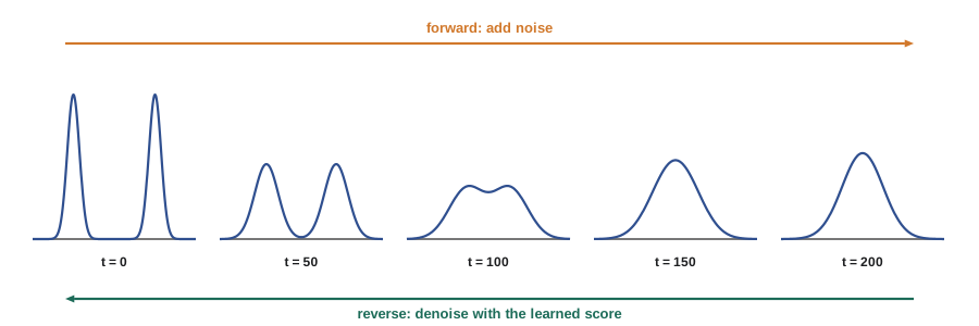
The samples recover both modes in equal proportion, centered near \(\pm 2\) with spread close to 0.3, from starting points that were pure noise. In a real model the exact score is replaced by a large network, usually a U-Net with attention or, increasingly, a transformer operating on patches (the diffusion transformer of William Peebles and Saining Xie, 2023), conditioned on the time step and on a text prompt through cross-attention. Classifier-free guidance (Jonathan Ho and Tim Salimans, 2022) trains the same network with and without the condition and extrapolates between the two predictions at sampling time, trading diversity for closer adherence to the prompt.

Sampling with hundreds of steps is slow, and much work has gone into reducing it: deterministic samplers such as DDIM (Jiaming Song, Chenlin Meng and Stefano Ermon, 2021), higher-order solvers of the equivalent ordinary differential equation, distillation into few-step students, and flow matching and rectified flow (Yaron Lipman and colleagues; Xingchao Liu and colleagues, both 2023), which learn straighter paths from noise to data and underlie several 2024–2026 image and video models. Diffusion and flow models now dominate image, video and audio generation, and they are being applied to molecules, proteins and robot actions.

Comparing the families

Each family makes a different trade. Autoregressive models factorize exactly and scale superbly, which is why they dominate text, but generation is sequential. VAEs are stable and give a latent space but blur. GANs are fast and sharp but unstable and prone to mode collapse. Diffusion models are stable, high quality and cover the data distribution well, but need many network evaluations unless distilled. Hybrids are common: latent diffusion uses an autoencoder plus diffusion, many image tokenizers use VAE-style models with GAN-style losses, and multimodal language models generate images by predicting tokens autoregressively or by driving a diffusion decoder. The responsible-use questions these capabilities raise, from deepfakes to copyright in training data, are taken up in lesson 12.

Worked examples