Recurrent networks and sequence modeling

Text, speech, sensor readings and prices arrive as sequences of varying length, in which order carries meaning and the relevant context can be far back. A feedforward network takes a fixed-size input and has no notion of order. Recurrent neural networks (RNNs) process a sequence one element at a time while carrying a hidden state that summarizes what they have seen, applying the same weights at every step. This lesson develops the simple RNN and its training by backpropagation through time, explains why plain RNNs struggle with long-range dependencies, and introduces the gated architectures (the LSTM and the GRU) that solved much of that problem and dominated sequence modeling from about 2014 to 2017. It closes with encoder-decoder models, whose limitations motivated the attention mechanism of lesson 8. AI-340 applies these models to language; the focus here is on the mechanisms.

The simple recurrent network

An RNN, in the form popularized by Jeffrey Elman (1990), updates a hidden state \(\mathbf{h}_t\) from the previous state and the current input,

with \(\mathbf{h}_0\) usually zero. The same matrices are used at every time step: weight sharing across time, the sequential analog of convolution's sharing across space. The state is a lossy summary of the whole history, of fixed size regardless of sequence length. Depending on the task, an output is produced at every step (tagging each word with its part of speech, predicting the next character), only at the end (classifying the sentiment of a review), or by a separate decoder (translation).

A language model is the canonical example. Trained to predict each next token from the ones before, with cross-entropy loss summed over positions, it assigns a probability to any sequence by the chain rule \(p(x_1, \dots, x_T) = \prod_t p(x_t \mid x_{<t})\), and it can generate text by sampling one token at a time and feeding it back as the next input. The quality of a language model is usually reported as perplexity, the exponential of the average cross-entropy per token: a perplexity of 20 means the model is, on average, as uncertain as if it were choosing uniformly among 20 tokens.

Backpropagation through time

Unrolling the recurrence over T steps turns the RNN into a deep feedforward network with T layers that share weights. Backpropagation through time (BPTT, described by Paul Werbos in 1990) runs ordinary backpropagation on this unrolled graph: the forward pass computes and stores every hidden state, and the backward pass walks from the last step to the first, accumulating gradients for the shared matrices from every step. Because a hidden state influences the loss both through its own output and through all later states, its adjoint is the sum of the two: \(\bar{\mathbf{h}}_t = W_{hy}^{\top}\bar{\mathbf{s}}_t + \bigl(\partial \mathbf{h}_{t+1}/\partial \mathbf{h}_t\bigr)^{\top}\bar{\mathbf{h}}_{t+1}\).

Long sequences make full BPTT expensive in memory, since every state must be stored. Truncated BPTT splits the sequence into chunks of, say, 50 to 200 steps, carries the hidden state forward across chunk boundaries but stops gradients there. The model can still carry information further than the truncation length, but it receives no gradient signal teaching it to do so.

# A character-level RNN trained by backpropagation through time on a short repeating text.
import numpy as np
rng = np.random.default_rng(466)
text = "the cat sat on the mat. " * 20
chars = sorted(set(text)); V = len(chars); ix = {c: i for i, c in enumerate(chars)}
data = np.array([ix[c] for c in text])
H, T, lr = 48, 24, 0.1
Wxh = rng.normal(0, 0.1, (V, H)); Whh = rng.normal(0, 0.1, (H, H)); Why = rng.normal(0, 0.1, (H, V))
bh, by = np.zeros(H), np.zeros(V)
def step(inputs, targets, hprev):
    hs = {-1: hprev}; ps = {}; loss = 0.0
    for t in range(len(inputs)):                       # forward through T time steps
        hs[t] = np.tanh(Wxh[inputs[t]] + hs[t - 1] @ Whh + bh)
        s = hs[t] @ Why + by; s -= s.max()
        ps[t] = np.exp(s) / np.exp(s).sum()
        loss -= np.log(ps[t][targets[t]])
    grads = [np.zeros_like(a) for a in (Wxh, Whh, Why, bh, by)]
    dWxh, dWhh, dWhy, dbh, dby = grads; dh_next = np.zeros(H)
    for t in reversed(range(len(inputs))):             # backward through time
        ds = ps[t].copy(); ds[targets[t]] -= 1
        dWhy += np.outer(hs[t], ds); dby += ds
        dh = ds @ Why.T + dh_next
        dz = (1 - hs[t] ** 2) * dh
        dWxh[inputs[t]] += dz; dWhh += np.outer(hs[t - 1], dz); dbh += dz
        dh_next = dz @ Whh.T
    for g in grads:
        np.clip(g, -5, 5, out=g)                       # clip to tame exploding gradients
    return loss / len(inputs), grads, hs[len(inputs) - 1]
mem = [np.zeros_like(a) for a in (Wxh, Whh, Why, bh, by)]
h = np.zeros(H); p = 0
for it in range(1, 1501):
    if p + T + 1 >= len(data): p, h = 0, np.zeros(H)
    loss, grads, h = step(data[p:p + T], data[p + 1:p + T + 1], h)
    for P, G, M in zip((Wxh, Whh, Why, bh, by), grads, mem):
        M += G * G; P -= lr * G / np.sqrt(M + 1e-8)     # AdaGrad
    p += T
    if it in (1, 100, 500, 1500):
        print(f"iteration {it:4}: loss per character {loss:.3f}")
h = np.zeros(H); c = ix["t"]; out = "t"
for _ in range(40):                                    # generate greedily from "t"
    h = np.tanh(Wxh[c] + h @ Whh + bh); c = int(np.argmax(h @ Why + by)); out += chars[c]
print("generated:", repr(out))

iteration    1: loss per character 2.394
iteration  100: loss per character 0.044
iteration  500: loss per character 0.004
iteration 1500: loss per character 0.001
generated: 'the cat sat on the mat. the cat sat on th'

On this deliberately easy text, the loss per character falls from about \(\log 11 \approx 2.4\) (uniform guessing over 11 distinct characters) to near zero, and the network reproduces the sentence. Andrej Karpathy's 2015 essay on the unreasonable effectiveness of RNNs showed the same simple model, scaled up and trained on Shakespeare, Wikipedia or source code, generating text with plausible spelling, syntax and indentation, a striking early demonstration of what next-token prediction can learn.

Vanishing and exploding gradients

The gradient of a late state with respect to an early one is a product of Jacobians,

one factor per time step. If the largest singular value of \(W_{hh}\), times the tanh slopes, is below 1, this product shrinks exponentially in \(T - t\) and the network cannot learn that something far back matters. If it is above 1, the product can grow exponentially and a single update can be catastrophic. Yoshua Bengio, Patrice Simard and Paolo Frasconi (1994) and Sepp Hochreiter (1991) identified this as the fundamental difficulty of training RNNs on long-range dependencies; Razvan Pascanu, Tomas Mikolov and Bengio (2013) analyzed it geometrically and proposed gradient norm clipping for the exploding case, which the character model above uses (clipping each element is a simpler variant).

# How the gradient of h_T with respect to h_t behaves as the time gap grows, for a tanh RNN.
import numpy as np
rng = np.random.default_rng(466)
n, T = 32, 60
for radius in (0.8, 1.0, 1.5):
    W = rng.normal(size=(n, n)); W *= radius / max(abs(np.linalg.eigvals(W)))   # set spectral radius
    U = rng.normal(0, 0.5, (n, 1))
    h = np.zeros(n); J = np.eye(n); norms = {}
    xs = rng.normal(size=T)
    for t in range(1, T + 1):
        h = np.tanh(W @ h + U[:, 0] * xs[t - 1])
        J = np.diag(1 - h ** 2) @ W @ J          # Jacobian d h_t / d h_0 by the chain rule
        if t in (1, 10, 30, 60):
            norms[t] = np.linalg.norm(J, 2)
    print(f"spectral radius {radius}: ||dh_t/dh_0|| at t = 1, 10, 30, 60: " + "  ".join(f"{norms[t]:.2e}" for t in (1, 10, 30, 60)))

spectral radius 0.8: ||dh_t/dh_0|| at t = 1, 10, 30, 60: 1.13e+00  2.10e-02  1.38e-06  1.15e-12
spectral radius 1.0: ||dh_t/dh_0|| at t = 1, 10, 30, 60: 1.75e+00  3.66e-01  8.69e-03  3.09e-06
spectral radius 1.5: ||dh_t/dh_0|| at t = 1, 10, 30, 60: 2.72e+00  2.92e+01  2.30e+01  4.68e+00

The output shows the exponential behavior. With spectral radius 0.8, the sensitivity of the state to its value 60 steps earlier is negligible; at 1.5 it is far larger (the tanh slopes eventually rein it in, since saturated units pass little gradient, which is another way gradients die). Clipping deals with explosions; vanishing needs an architectural fix.

Long short-term memory

The long short-term memory (LSTM) of Sepp Hochreiter and Jürgen Schmidhuber (1997), with the forget gate added by Felix Gers, Schmidhuber and Fred Cummins (2000), adds a separate cell state \(\mathbf{c}_t\) that is updated additively under the control of gates. Each gate is a sigmoid layer whose outputs between 0 and 1 multiply another vector elementwise:

The forget gate decides how much of the old memory to keep, the input gate how much of the new candidate \(\mathbf{g}_t\) to write, and the output gate how much of the memory to expose as the hidden state. The key is the additive update of \(\mathbf{c}_t\): the gradient from \(\mathbf{c}_t\) to \(\mathbf{c}_{t-1}\) is just \(\mathbf{f}_t\), elementwise, with no matrix multiplication and no tanh squashing. When the forget gate is near 1, gradient flows back through many steps almost unchanged. This constant error carousel, as Hochreiter and Schmidhuber called it, is the same idea as the identity path of a residual network, discovered nearly twenty years earlier for depth in time. Initializing the forget-gate bias to about 1, so the cell remembers by default, is a standard trick (Rafal Jozefowicz and colleagues, 2015).

# One LSTM cell step, written out gate by gate.
import numpy as np
rng = np.random.default_rng(466)
d, n = 3, 4                                        # input size, hidden size
W = rng.normal(0, 0.5, (4 * n, d + n)); b = np.zeros(4 * n)
b[n:2 * n] = 1.0                                   # forget-gate bias of 1: remember by default
sig = lambda z: 1 / (1 + np.exp(-z))
def lstm_step(x, h, c):
    z = W @ np.concatenate([x, h]) + b
    i, f, o, g = sig(z[:n]), sig(z[n:2 * n]), sig(z[2 * n:3 * n]), np.tanh(z[3 * n:])
    c_new = f * c + i * g                          # additive memory update
    h_new = o * np.tanh(c_new)
    return h_new, c_new, (i, f, o, g)
h, c = np.zeros(n), np.array([2.0, -1.0, 0.5, 0.0])  # a cell already holding some memory
x = np.array([1.0, 0.0, -1.0])
h, c2, (i, f, o, g) = lstm_step(x, h, c)
for name, v in (("input gate i", i), ("forget gate f", f), ("output gate o", o), ("candidate g", g)):
    print(f"{name:14} {np.round(v, 3)}")
print(f"old cell c     {c}")
print(f"new cell c     {np.round(c2, 3)}")
print(f"hidden h       {np.round(h, 3)}")
print("parameters in this LSTM layer:", W.size + b.size, "= 4 x (hidden x (input + hidden) + hidden)")

input gate i   [0.526 0.245 0.384 0.514]
forget gate f  [0.674 0.873 0.87  0.655]
output gate o  [0.234 0.727 0.37  0.512]
candidate g    [-0.334 -0.201  0.08   0.286]
old cell c     [ 2.  -1.   0.5  0. ]
new cell c     [ 1.173 -0.923  0.466  0.147]
hidden h       [ 0.193 -0.529  0.161  0.075]
parameters in this LSTM layer: 128 = 4 x (hidden x (input + hidden) + hidden)

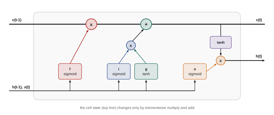
The gated recurrent unit (GRU) of Kyunghyun Cho and colleagues (2014) merges the cell and hidden states and uses two gates, an update gate that interpolates between the old state and a candidate, and a reset gate that controls how much of the old state the candidate sees. It has three quarters of the LSTM's parameters and performs comparably on many tasks; Junyoung Chung and colleagues (2014) and later larger studies found neither consistently better. Both remain in use where memory and latency are tight, such as on-device speech recognition, and in time-series forecasting.

Architectural variations

Bidirectional RNNs run one RNN forward and another backward over the sequence and concatenate their states, so each position's representation reflects both past and future context; they suit tagging and encoding tasks where the whole sequence is available, but not generation. Stacked or deep RNNs feed one layer's hidden states as the next layer's inputs, typically two to four layers, often with residual connections and dropout between layers. Sequence models can also be built from convolutions: temporal convolutional networks with dilated causal convolutions (lesson 6) process all positions in parallel and have competed well with LSTMs on many benchmarks (Shaojie Bai, Zico Kolter and Vladlen Koltun, 2018).

Encoder-decoder models and the bottleneck

For mapping one sequence to another of different length, such as translation, Ilya Sutskever, Oriol Vinyals and Quoc Le (2014) and Cho and colleagues (2014) introduced the encoder-decoder or sequence-to-sequence model. An encoder RNN reads the source sentence and its final state becomes the initial state of a decoder RNN, which generates the target one token at a time, each step conditioned on the previous output. During training the decoder is fed the true previous token (teacher forcing); at inference it is fed its own predictions, usually chosen by beam search, which keeps several partial hypotheses. Sutskever and colleagues' four-layer LSTM model approached the best phrase-based translation systems on English to French, and reversing the source sentence helped, a hint that the model struggled to carry information across long distances.

The weakness is the bottleneck: the entire source sentence must be squeezed into one fixed-size vector, and performance drops sharply on long sentences. Dzmitry Bahdanau, Kyunghyun Cho and Yoshua Bengio (2015) let the decoder look back at all encoder states at every step, computing a weighted average whose weights depend on how relevant each source position is to the current output. This was the attention mechanism. It removed the bottleneck, produced interpretable soft alignments between words in the two languages, and became the starting point for the transformer of lesson 8, which keeps the attention and discards the recurrence.

Why recurrence lost ground

RNNs have two structural limitations that attention overcomes. They are sequential: step t cannot be computed until step t − 1 is done, so training cannot be parallelized across positions, which wastes the parallelism of GPUs and limits how much data can be processed. And information between distant positions must pass through many state updates, so even with gating, long-range dependencies remain hard to learn. Transformers compute all positions in parallel during training and connect any two positions in one step. Recurrence is not gone, though: state space models such as S4 (Albert Gu, Karan Goel and Christopher Ré, 2022) and Mamba (Albert Gu and Tri Dao, 2023), and linear-recurrence models such as RWKV, train in parallel like convolutions or attention but run like RNNs at inference with constant memory per step, and hybrid models that mix such layers with attention are an active area as of 2026. AI-410 discusses them in the context of long-context language models.

Worked examples