
BIOL-499 · Lesson 5 of 12 · 19 min
Designing the study: replication, controls, sampling and power
▶ Video coming soon A video version of this lesson is on the way.
Study design decides what a project can and cannot conclude. No statistical analysis, however clever, can rescue data from a design that confounds the treatment with something else or that has too few independent replicates. This lesson covers the design decisions Priya made between February and April 2025: what her experimental units were, how she dealt with the fact that she could not choose which wetlands were fenced, how many replicates she needed, what she would measure and when, and how she checked whether her design had enough power to detect the effect she expected.
Many of these ideas were introduced in BIOL-430 Field Ecology and in statistics courses. Here they are applied to one real decision after another, which is how they are used in research.
Experimental units and replication
The experimental unit is the smallest unit to which a treatment is independently applied. In Priya's study, the treatment, cattle exclusion, was applied to whole wetlands: a fence surrounded each wetland margin. The experimental unit was therefore the wetland, not the tadpole, the dip-net sweep or the water sample. She would take many measurements in each wetland, but those measurements are subsamples, and they tell her about that wetland, not about the effect of fencing in general.
Treating subsamples as independent replicates is called pseudoreplication, a term popularized by Stuart Hurlbert in 1984. If Priya had counted tadpoles in 20 sweeps at one fenced and 20 at one grazed wetland and compared the 20 against the 20, any difference could be due to the two wetlands differing in countless ways unrelated to fencing. Her sample size for the fencing comparison was 12 pairs of wetlands, not hundreds of sweeps. Subsamples are still valuable: averaging many sweeps gives a more precise estimate for each wetland, which reduces noise in the comparison.
| Project | Treatment applied to | Experimental unit | Subsamples |
|---|---|---|---|
| Priya: cattle exclusion | Whole wetland margins | Wetland (12 pairs) | Dip-net sweeps, water samples, recorder nights |
| Tomás: temperature | Growth chambers | Chamber, unless each jar has its own temperature control | Jars and individual Daphnia within a chamber |
| Aisha: manure | Fields | Field | Soil cores and bacterial isolates within a field |
Tomás's case is a common trap in lab projects. If all 18 jars at 24 degrees sit in one incubator and all 18 at 28 degrees in another, temperature is confounded with incubator: a difference in light, humidity or a faulty thermostat would look like a temperature effect. With only two incubators available, Tomás solved this by running the experiment in three rounds, swapping the temperatures between incubators each round, so that each temperature was tested in more than one incubator and round could be included in the analysis.
Controls and confounding
A control is a comparison that shows what happens without the treatment. Priya's controls were grazed wetlands. The danger in an observational comparison is confounding: a variable related both to the treatment and to the response. The ranch had not fenced wetlands at random. It fenced wetlands near water troughs where cattle damage was worst, and wetlands with better access for fencing crews. Fenced and grazed wetlands might therefore differ in size, depth or surrounding land use, any of which could affect frogs.
The station's design reduced confounding in three ways. First, wetlands were paired within the same pasture, so each pair shared soils, weather, cattle herd and management history. Second, pairs were matched on wetland area and permanence class before fencing. Third, the station had measured water chemistry and vegetation at every wetland for two years before fencing and two years after, so that pre-existing differences could be checked. Priya used those baseline data to show that fenced and grazed wetlands had similar turbidity before fencing, which strengthened the case that any later difference was caused by the fences.
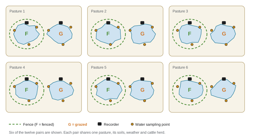
Randomization is the strongest protection against confounding, because it makes the treatment independent of every other variable on average. Priya could not randomize fencing, which had been done years earlier. She acknowledged this as a limitation, relied on pairing and baseline data to reduce it, and was careful to write that her results showed differences associated with fencing that were consistent with a causal effect, rather than claiming proof. In her lab-based project, Tomás could randomize: he assigned jars to temperatures with a random number generator and recorded the seed so that the assignment could be reproduced.
Choosing what to measure
Each prediction needs at least one response variable, and each response needs a method, a unit and a schedule. Priya also measured covariates, variables that are not the focus but might explain variation, such as wetland area, depth and water temperature. Including them in the analysis can reduce noise and account for differences between pairs.
| Variable | Method | Schedule | Role |
|---|---|---|---|
| Turbidity (NTU) | Calibrated portable turbidimeter, three readings around each margin | Four visits, late April to late June | Response (aim 1), mechanism |
| Emergent vegetation cover | Point-intercept along four fixed transects | Once, mid-June | Response (aim 1) |
| Calling activity | Automated recorder, chorus index scored for 30 nights | Recorders run 20 April to 31 May | Response (aim 2) |
| Tadpole density | Ten standardized dip-net sweeps per wetland | Two visits, early and mid-June | Response (aim 2) |
| eDNA detection | Three 1-liter water samples filtered on site, qPCR in triplicate | One visit, mid-May | Response (aim 3) |
| Area, depth, water temperature | GPS outline, staff gauge, logger | Each visit | Covariates |
Measurement methods should be standardized so that differences reflect the wetlands, not the observer. Priya used the same sweep length, net and posture at every wetland, sampled in a fixed order around each margin, and visited the two wetlands in a pair on the same day, alternating which she visited first. Calling was scored from recordings by listening to a two-minute segment beginning 30 minutes after sunset each night and assigning a calling index from 0 (no frogs) to 3 (a full chorus with continuous, overlapping calls), a scale widely used in amphibian monitoring programs. To reduce bias, recordings were renamed with codes so that Priya did not know whether each recording came from a fenced or grazed wetland when she scored it. This is called blinding, and it guards against the unconscious tendency to hear what one expects.
Sample size and statistical power
Statistical power is the probability that a study will detect an effect of a given size if it truly exists. Power depends on four things: the size of the effect, the variability of the data, the number of independent replicates and the significance threshold. A study with low power is likely to miss real effects, and when it does find one, the estimate is likely to be exaggerated. Calculating power before collecting data tells you whether your design is worth carrying out, or whether you need more replicates, less variable measurements or a different question.
Dr. Szabo's question at the proposal presentation was whether 12 pairs were enough. To answer it, Priya needed an expected effect size and an estimate of variability. From the literature and from pilot counts at the station the year before, she expected fenced wetlands to have about 1.6 times as many tadpoles as grazed wetlands, and she estimated the standard deviation of the log ratio of tadpole densities within pairs as about 0.6. She then estimated power by simulation: generate many imaginary data sets with those properties, analyze each one, and count how often the test detects the effect.
# Power by simulation for a paired design: log(fenced / grazed) tadpole density per pair.
import numpy as np
from scipy import stats
rng = np.random.default_rng(499)
effect = np.log(1.6)     # fenced wetlands 1.6 times as many tadpoles
sd = 0.60                # SD of the within-pair log ratio, from pilot counts
for n in (6, 8, 10, 12, 16, 20, 24):
    d = rng.normal(effect, sd, size=(4000, n))
    p = stats.ttest_1samp(d, 0, axis=1).pvalue
print(f"{n:2d} pairs: power = {np.mean(p < 0.05):.2f}")6 pairs: power = 0.34 8 pairs: power = 0.48 10 pairs: power = 0.60 12 pairs: power = 0.69 16 pairs: power = 0.84 20 pairs: power = 0.91 24 pairs: power = 0.95
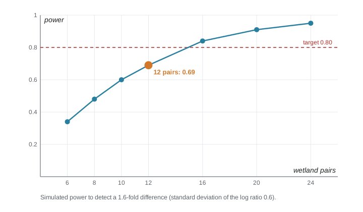
With 12 pairs, the simulation gave a power of about 0.69: if the true effect were a 1.6-fold increase, the study would detect it about 7 times in 10. The conventional target is 0.80, which would need about 15 pairs. Only 12 pairs existed, so adding replicates was impossible. Priya considered three responses. She could reduce variability by taking more sweeps per visit and averaging two visits, which would lower the standard deviation. She could accept the limitation and report the effect with a confidence interval, so that even a non-significant result would show which effect sizes were and were not plausible. And she could note that larger effects would be detected reliably: a 1.8-fold difference would be detected about 87 times in 100 with 12 pairs. She did all three, and her revised proposal stated the power calculation openly.
Power analysis is most useful before a study. Calculating power after a study, using the effect size you observed, is generally uninformative, because it follows directly from the p-value. If a study finds no significant effect, the confidence interval is the better guide to what the data rule out.
Sampling schedules and timing
In field biology, when you sample can matter as much as where. Chorus frogs call from snowmelt into late May in central Alberta and Minnesota, eggs hatch within one to two weeks depending on temperature, and tadpoles metamorphose in roughly six to ten weeks. Sampling tadpoles too early would miss late breeders; too late, and some wetlands would have dried or tadpoles would have left. Priya used degree-days, accumulated warmth above a threshold, from the station's weather data to time her tadpole visits, and visited each pair on the same day so that time of season was the same for both wetlands.
Lab projects have equivalent timing issues: the age of cultures, the time of day of measurements and the batch of reagents. Recording these and spreading treatments evenly across them, rather than doing all of one treatment on Monday and another on Friday, prevents hidden confounding.
Worked problem
Finding the experimental unit
Aisha samples 10 manured and 10 unmanured fields. In each field she takes 5 soil cores and isolates 8 bacteria per core, testing each isolate for resistance. She finds 240 resistant isolates out of 400 from manured fields and 120 out of 400 from unmanured fields, and proposes a chi-square test on the 800 isolates. What is wrong, and what should she do?
Show solution
- The treatment, manure, is applied to whole fields, so the field is the experimental unit and n is 10 per group.
- Cores and isolates are subsamples; isolates from the same field are not independent, because they share soil, history and possibly clonal bacteria.
- A chi-square test on 800 isolates treats them as independent, which is pseudoreplication and greatly overstates the evidence.
- Instead, compute the proportion of resistant isolates in each field, giving 10 values per group, and compare the groups with a test on field-level values, or use a model with field as a random effect.
Answer: The analysis should be based on 10 fields per group, not 800 isolates. Field-level proportions, or a mixed model that includes field as a random effect, respect the design.
Common mistakes
MistakeMore measurements always mean more replication.
InsteadOnly independent applications of the treatment are replicates; subsamples improve precision within units but do not add replicates.
MistakePairing is unnecessary if the sample is large enough.
InsteadPairing removes variation shared within pairs, increasing power and reducing confounding for the same number of units.
MistakePower should be calculated after the study from the observed effect.
InsteadCalculate power before a study; afterwards, report confidence intervals.
MistakeObservational comparisons cannot be useful.
InsteadWith pairing, baseline data and careful wording, observational designs provide valuable evidence, though weaker than randomized experiments.
Summary and key terms
- The experimental unit is the smallest unit to which a treatment is independently applied; subsamples within units are not replicates.
- Pseudoreplication treats subsamples as replicates and exaggerates the evidence.
- Controls, pairing, matching and baseline data reduce confounding when randomization is not possible; randomize whenever you can.
- Standardize methods, measure covariates and blind observers to treatment where possible.
- Power depends on effect size, variability, replication and the significance threshold, and can be estimated by simulation before a study.
- Time sampling to the biology of the organism and spread treatments evenly across time, batches and observers.
- Experimental unit
- The smallest unit to which a treatment is independently applied.
- Pseudoreplication
- Treating non-independent subsamples as if they were independent replicates.
- Confounding variable
- A variable related to both the treatment and the response that can create a false appearance of a treatment effect.
- Blinding
- Keeping the person making measurements unaware of which treatment each sample received.
- Statistical power
- The probability that a study detects an effect of a given size if it exists.
- Covariate
- A variable measured because it may explain variation in the response, though it is not the main focus.
Practice problems
Work each problem on paper first, then reveal the answer to check.
A greenhouse study has 4 benches, 2 heated and 2 unheated, with 25 pots per bench. What is the experimental unit and n per treatment?
Show answer
If heating is applied per bench, the bench is the unit and n is 2 per treatment, which is very low.
Why did Priya visit both wetlands in a pair on the same day?
Show answer
So that time of season, weather and frog development were the same for both, preventing timing from confounding the comparison.
A design has power 0.45 for the expected effect. Name two ways to improve it.
Show answer
Increase independent replicates, reduce variability by better measurement or more subsamples, use pairing or blocking, or focus on a larger expected effect.
What is blinding, and why did Priya use it?
Show answer
Scoring recordings without knowing the treatment, to avoid unconscious bias in judging calling intensity.
Lesson quiz · 5 questions
Score 60% or more to complete this lesson.
Create a free account to save your progress, take quizzes and earn a certificate.