
AI-480 · Lesson 9 of 12 · 24 min
Pipeline parallelism and 3D parallelism
Pipeline parallelism divides a model by depth: the first group of layers goes on one device, the next group on another, and so on, with activations flowing from stage to stage like work along an assembly line. Unlike tensor parallelism, it communicates only at the boundaries between stages, and only the activations of one micro-batch at a time, so it tolerates the slower links between servers. Its difficulty is idle time: a stage cannot start until the previous one hands it work, and the backward pass flows in the opposite direction. This lesson explains pipeline schedules from GPipe to interleaved and zero-bubble designs, how to calculate and reduce the pipeline bubble, how stages are balanced, and how tensor, pipeline and data parallelism combine into the 3D parallelism used to train the largest models.
The naive pipeline and the bubble
Suppose a model is split into \(p\) stages on \(p\) devices. If a whole batch flows through in one piece, only one device works at a time: stage 1 runs its forward pass while the others wait, then stage 2, and so on, followed by the backward pass in reverse. Each device is idle for a fraction \((p-1)/p\) of the time. Splitting the batch into \(m\) micro-batches lets the stages work on different micro-batches at once. Stage 1 starts micro-batch 2 as soon as it passes micro-batch 1 to stage 2. Idle time remains only while the pipeline fills at the start and drains at the end, a period called the pipeline bubble.
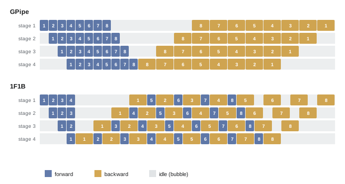
GPipe, introduced by Huang and colleagues at Google in 2019, runs all \(m\) forward passes, then all \(m\) backward passes, then a synchronous optimizer step. With forward and backward times per micro-batch per stage of \(t_f\) and \(t_b\), the bubble lasts \((p-1)(t_f + t_b)\) out of a total of \((m + p - 1)(t_f + t_b)\), so the bubble fraction is:
To keep the bubble small, \(m\) must be large compared with \(p\): with 8 stages, 64 micro-batches give a bubble of about 10 %. But GPipe stores the activations of all \(m\) micro-batches on each stage until their backward passes run, so memory grows with \(m\), working against the very thing that shrinks the bubble.
One forward, one backward
The 1F1B schedule, used in PipeDream-Flush and Megatron-LM, reorders the work. Each stage runs a few warm-up forward passes, enough to fill the pipeline, then alternates one forward and one backward pass, and finally drains the remaining backward passes. Because each micro-batch's backward pass starts as soon as possible, a stage never holds more than about \(p\) micro-batches of activations, regardless of \(m\). The bubble is the same as GPipe's, but memory no longer limits the number of micro-batches.
import numpy as np
# Simulate pipeline schedules with p stages and m micro-batches.
# Forward of one micro-batch on one stage takes 1 unit; backward takes 2 units.
def simulate(p, m, schedule):
    free = [0] * p                      # time each stage becomes free
    f_done = np.zeros((p, m)); b_done = np.zeros((p, m))
    inflight = [0] * p; peak = [0] * p
    order = []
    for s in range(p):
        if schedule == "gpipe":
            ops = [("F", i) for i in range(m)] + [("B", i) for i in reversed(range(m))]
        else:                           # 1F1B: warm-up forwards, then alternate, then drain
            warm = min(p - s, m)
            ops = [("F", i) for i in range(warm)]
            f, b = warm, 0
            while b < m:
                ops.append(("B", b)); b += 1
                if f < m: ops.append(("F", f)); f += 1
        order.append(ops)
    idx = [0] * p
    while any(idx[s] < len(order[s]) for s in range(p)):
        progressed = False
        for s in range(p):
            if idx[s] >= len(order[s]): continue
            kind, i = order[s][idx[s]]
            if kind == "F":
                ready = f_done[s - 1, i] if s > 0 else 0
                if s > 0 and ready == 0: continue
                start = max(free[s], ready); f_done[s, i] = start + 1; free[s] = start + 1
                inflight[s] += 1; peak[s] = max(peak[s], inflight[s])
            else:
                if f_done[s, i] == 0: continue
                ready = b_done[s + 1, i] if s < p - 1 else f_done[s, i]
                if s < p - 1 and ready == 0: continue
                start = max(free[s], ready); b_done[s, i] = start + 2; free[s] = start + 2
                inflight[s] -= 1
            idx[s] += 1; progressed = True
        assert progressed
    total = max(free); busy = 3 * m
    return total, 1 - busy / total, peak[0]
for p, m in [(4, 4), (4, 16), (8, 8), (8, 64)]:
    for sch in ("gpipe", "1f1b"):
        total, bubble, peak = simulate(p, m, sch)
print(f"p={p} m={m:2d} {sch:5s}: step time {total:4.0f} bubble {bubble:5.1%} formula {(p-1)/(m+p-1):5.1%} peak activations on stage 0: {peak}")p=4 m= 4 gpipe: step time 21 bubble 42.9% formula 42.9% peak activations on stage 0: 4 p=4 m= 4 1f1b : step time 21 bubble 42.9% formula 42.9% peak activations on stage 0: 4 p=4 m=16 gpipe: step time 57 bubble 15.8% formula 15.8% peak activations on stage 0: 16 p=4 m=16 1f1b : step time 57 bubble 15.8% formula 15.8% peak activations on stage 0: 4 p=8 m= 8 gpipe: step time 45 bubble 46.7% formula 46.7% peak activations on stage 0: 8 p=8 m= 8 1f1b : step time 45 bubble 46.7% formula 46.7% peak activations on stage 0: 8 p=8 m=64 gpipe: step time 213 bubble 9.9% formula 9.9% peak activations on stage 0: 64 p=8 m=64 1f1b : step time 213 bubble 9.9% formula 9.9% peak activations on stage 0: 8
The simulator reproduces the bubble formula exactly for both schedules, and shows the difference that matters: with 8 stages and 64 micro-batches, GPipe's first stage holds activations for all 64 micro-batches at its peak, while 1F1B holds only 8.
Interleaved and zero-bubble schedules
Narayanan and colleagues (2021) reduced the bubble further with the interleaved 1F1B schedule. Instead of one contiguous block of layers, each device holds \(v\) smaller, non-adjacent chunks, called virtual stages; for example, with 4 devices and 16 layers, device 1 might hold layers 1–2 and 9–10. Micro-batches loop through the devices \(v\) times. Each stage's work per micro-batch shrinks by a factor of \(v\), and the bubble shrinks with it:
The cost is \(v\) times more point-to-point communication, since activations cross between devices more often. More recent schedules attack the bubble directly. The zero-bubble schedules of Qi and colleagues (2023) split each backward pass into two parts: computing gradients with respect to the inputs, which the previous stage is waiting for, and computing gradients with respect to the weights, which can be deferred to fill idle slots. DeepSeek-V3's DualPipe schedule feeds micro-batches from both ends of the pipeline and overlaps computation with communication, including the all-to-all traffic of its experts.
Worked problem
Choosing the number of micro-batches
A model is split into 16 pipeline stages. The global batch per data-parallel replica is 256 sequences, and memory allows a micro-batch of 2 sequences. What is the bubble fraction with plain 1F1B, and with an interleaved schedule using 4 virtual stages per device?
Show solution
- Micro-batches per step: \(m = 256 / 2 = 128\).
- Plain 1F1B: \((16 - 1)/(128 + 16 - 1) = 15/143 \approx 10.5\) %.
- Interleaved with \(v = 4\): \(15/(4 \times 128) \approx 2.9\) %.
- The interleaved schedule needs four times as many stage-to-stage transfers.
Answer: About 10.5 % idle time with 1F1B and about 2.9 % with four-way interleaving, worth the extra point-to-point traffic if links are fast enough.
Balancing stages
A pipeline runs at the speed of its slowest stage, so stages must be balanced in both compute and memory. Transformer blocks are uniform, which helps, but the first stage also holds the token embedding and the last stage holds the output layer and loss, whose vocabulary-sized matrices can equal several transformer layers in cost. Common remedies place fewer transformer layers on the first and last stages, or treat the embedding and output as separate stages. Memory is unbalanced too: under 1F1B, the first stage holds activations for about \(p\) micro-batches and the last stage for only one, so the first stages may need activation recomputation while the last do not. Frameworks also must handle details such as tying the input and output embeddings, which live on different stages, by synchronizing their gradients.
Communication in pipelines
Between stages, each micro-batch passes an activation tensor of size \(s \times b \times h\) forward and a gradient of the same size backward, using point-to-point send and receive operations. For a micro-batch of one 4,096-token sequence with hidden size 8,192 in BF16, that is 67 MB in each direction, which takes under 2 ms over a 50 GB/s network link and can be overlapped with computation. This modest, predictable traffic is why pipeline stages are usually placed on different servers, while the much heavier tensor-parallel traffic stays inside servers.
3D parallelism
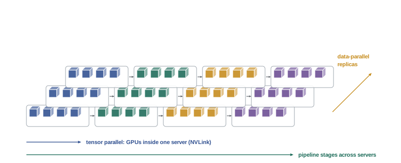
The largest models combine all three dimensions. With tensor-parallel degree \(t\), pipeline-parallel degree \(p\) and data-parallel degree \(d\), the cluster uses \(N = t \times p \times d\) devices:
- Tensor parallelism inside each server, over NVLink, splitting each layer across typically 8 GPUs.
- Pipeline parallelism across servers, splitting the depth of the model into stages.
- Data parallelism, usually with sharding, across replicas of the whole tensor-and-pipeline group, using the remaining devices.
Context and expert parallelism add further dimensions where needed. Meta trained Llama 3 405B on up to 16,384 H100 GPUs using 8-way tensor parallelism, 16-way pipeline parallelism and 128-way sharded data parallelism, adding context parallelism for long-context training, and reported 38 to 43 % MFU. The mapping onto hardware matters as much as the degrees: ranks are ordered so that tensor-parallel groups share a server, pipeline neighbors sit close together in the network, and data-parallel groups span the cluster, where their gradient reductions can overlap with computation.
| Constraint | Effect on the configuration |
|---|---|
| Model state must fit | Sets the minimum product of t, p and sharding |
| Tensor parallelism needs fast links | Caps t at the NVLink domain, often 8 |
| Bubble falls with micro-batches per replica | Large d leaves fewer micro-batches per pipeline |
| Global batch is fixed by convergence | d × m × micro-batch must equal the global batch |
| Data-parallel traffic grows with model size per replica | Prefer sharding and overlap for large replicas |
Choosing a configuration is a constrained search, and several tools help. Performance models estimate step time from compute, memory and communication; automatic planners such as Alpa search the space; and in practice engineers start from published configurations for similar models and hardware, then profile and adjust.
Pipelines and the global batch
Pipeline parallelism interacts with the global batch size. To keep the bubble small, each pipeline needs many micro-batches per step, but the global batch is set by convergence and divided among data-parallel replicas. A cluster with many replicas leaves each pipeline few micro-batches and a large bubble. For example, with a global batch of 1,024 sequences, micro-batches of one sequence and 8 pipeline stages, 64 replicas give each pipeline 16 micro-batches and a bubble of about 30 %, while 16 replicas give 64 micro-batches and a bubble of about 10 %, but take four times longer per step. This tension is one reason very large runs adopt interleaved or zero-bubble schedules, and why the global batch is sometimes increased later in training once the critical batch size has grown.
Common mistakes
MistakeUsing too few micro-batches for the number of stages.
InsteadKeep m much larger than p, or interleave.
MistakeUsing GPipe scheduling with many micro-batches.
InsteadUse 1F1B to bound activation memory.
MistakeSplitting layers evenly when the first and last stages are heavier.
InsteadAccount for embeddings, output layer and loss.
MistakePlacing pipeline stages inside a server and tensor parallelism across servers.
InsteadPut tensor parallelism on NVLink and pipelines across nodes.
MistakeChoosing degrees without checking the global batch.
InsteadEnsure d × m × micro-batch matches the target batch.
Summary and key terms
- Pipeline parallelism splits a model by depth into stages.
- Micro-batches let stages work concurrently, leaving a fill-and-drain bubble.
- The bubble fraction is (p − 1)/(m + p − 1).
- 1F1B keeps the bubble but bounds activations to about p micro-batches.
- Interleaved and zero-bubble schedules shrink the bubble further.
- Stages must balance compute and memory, including embeddings and the loss.
- 3D parallelism combines tensor, pipeline and data parallelism mapped onto the network.
- Pipeline stage
- Contiguous group of layers on one device.
- Pipeline bubble
- Idle time while a pipeline fills and drains.
- GPipe
- Schedule running all forwards, then all backwards.
- 1F1B
- Schedule alternating one forward and one backward.
- Virtual stage
- One of several model chunks held by a device.
- Interleaved schedule
- Pipeline using multiple virtual stages per device.
- Zero-bubble schedule
- Splitting backward work to fill idle slots.
- Point-to-point communication
- Sends and receives between two devices.
- 3D parallelism
- Combined tensor, pipeline and data parallelism.
- Rank mapping
- Assignment of parallel groups to physical devices.
Practice problems
Work each problem on paper first, then reveal the answer to check.
Bubble fraction for 4 stages and 12 micro-batches?
Show answer
3/15 = 20 %.
How many micro-batches keep the bubble near 5 % with 8 stages?
Show answer
About 133 (7/(m+7) = 0.05).
Why does GPipe need more memory than 1F1B?
Show answer
It holds activations for all m micro-batches.
Interleaved bubble for p = 8, m = 32, v = 2?
Show answer
7/64 ≈ 11 %.
What do zero-bubble schedules defer?
Show answer
Weight-gradient computation.
Why may the last stage be heavier?
Show answer
It holds the output layer and loss.
What passes between pipeline stages?
Show answer
Activations forward and gradients backward.
How many GPUs for t = 8, p = 12, d = 64?
Show answer
6,144.
Where should tensor-parallel groups be placed?
Show answer
Within a server on NVLink.
Name Llama 3 405B's tensor and pipeline degrees.
Show answer
8-way tensor, 16-way pipeline.
Lesson quiz · 5 questions
Score 60% or more to complete this lesson.
Create a free account to save your progress, take quizzes and earn a certificate.