
AI-480 · Lesson 1 of 12 · 25 min
The scale of modern AI training
Training a frontier language model is one of the largest computations people have ever run. A single training job can occupy tens of thousands of accelerators for months, read trillions of words, perform around \(10^{25}\) floating-point operations and draw tens of megawatts of electricity. Even models a thousand times smaller, the kind a university lab or a start-up trains, are too big for one chip: they must be split across many devices that cooperate through fast networks. This course explains how that works, from the transistor-level design of graphics processing units (GPUs) and other accelerators, through the numerical formats and memory budgets that decide what fits on a chip, to the parallelism strategies, networks, storage and software that turn thousands of chips into one training machine, and finally the energy and economics that shape what gets built. This first lesson sets the scene: what the training workload is, how to count its cost, and why scale has become the central engineering problem of modern AI.
What a training step does
Neural network training repeats one basic step billions of times. A mini-batch of examples, such as a few million tokens of text, flows forward through the network to produce predictions and a loss; the backward pass applies the chain rule to compute the gradient of the loss with respect to every parameter; and an optimizer such as Adam uses the gradients to update the parameters. Almost all of the arithmetic sits in matrix multiplications: the dense layers of a transformer, the projections inside attention, and the embedding and output layers. A matrix multiplication of an \(m \times k\) matrix by a \(k \times n\) matrix needs \(2mkn\) floating-point operations (one multiply and one add per term), so a network's cost is dominated by how many parameters each token touches.
This regular, massively parallel arithmetic is why AI training moved from general-purpose central processing units (CPUs) to GPUs and purpose-built accelerators. A CPU devotes much of its silicon to making a few threads run fast: branch prediction, out-of-order execution and large caches. A GPU devotes most of its silicon to thousands of simple arithmetic units that execute the same instruction on different data, which is exactly the shape of a matrix multiplication.
Counting training compute
For a dense transformer with \(N\) parameters trained on \(D\) tokens, a widely used approximation gives the total training compute:
The factor 6 comes from 2 operations per parameter per token in the forward pass (a multiply and an add) and about 4 in the backward pass, which computes gradients both with respect to activations and with respect to weights. The approximation ignores attention's dependence on sequence length, which adds a modest amount for typical context lengths, and the small cost of the optimizer update. It is accurate enough for planning: GPT-3, with 175 billion parameters trained on about 300 billion tokens, works out to about \(3.1 \times 10^{23}\) FLOPs, matching the figure its authors reported.
Note the difference between FLOPs, a count of operations, and FLOP/s (FLOPS), a rate. Hardware is rated in FLOP/s: an NVIDIA H100 SXM delivers about 989 teraFLOP/s (\(9.89 \times 10^{14}\)) of dense BF16 matrix arithmetic at its peak. Dividing the training compute by the sustained rate of the whole cluster gives the training time.
Worked problem
Estimating training time
A team plans to train a 13-billion-parameter model on 2 trillion tokens using 512 H100 GPUs (989 TFLOP/s peak each) and expects to sustain 40 % of peak. How long will training take?
Show solution
- Compute: \(C = 6 \times 13 \times 10^{9} \times 2 \times 10^{12} = 1.56 \times 10^{23}\) FLOPs.
- Sustained cluster rate: \(512 \times 989 \times 10^{12} \times 0.40 = 2.03 \times 10^{17}\) FLOP/s.
- Time: \(1.56 \times 10^{23} / 2.03 \times 10^{17} \approx 7.7 \times 10^{5}\) s.
- Convert: \(7.7 \times 10^{5} / 86{,}400 \approx 8.9\) days, or about 109,000 GPU-hours.
Answer: About 9 days of continuous training, roughly 109,000 GPU-hours, before allowing for failures and restarts.
Scaling laws
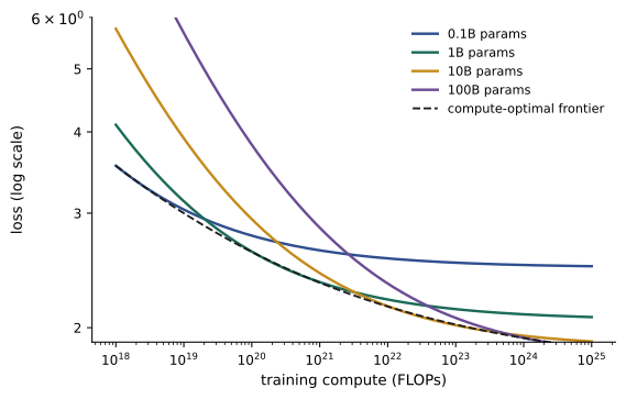
Why train such large models? Empirical scaling laws show that a language model's loss falls smoothly and predictably as a power law in parameters, data and compute. Kaplan and colleagues at OpenAI (2020) found that test loss improved steadily over seven orders of magnitude of compute. Hoffmann and colleagues at DeepMind (2022), in the Chinchilla paper, refined the picture: for a fixed compute budget, parameters and tokens should grow roughly in proportion, with about 20 training tokens per parameter giving the lowest loss. Their 70-billion-parameter Chinchilla, trained on 1.4 trillion tokens, outperformed the much larger 280-billion-parameter Gopher trained with the same compute.
Since then, many teams have deliberately trained smaller models on far more data than the compute-optimal ratio, because a smaller model is cheaper to serve to millions of users. Meta's Llama 3 8B, for example, was trained on about 15 trillion tokens, close to 1,900 tokens per parameter. The training budget is only one part of the total cost; inference, which runs every time someone uses the model, often dominates over the model's lifetime.
import numpy as np
# Training compute: C = 6 N D floating-point operations
def train_flops(params, tokens):
    return 6.0 * params * tokens
# A compute-optimal (Chinchilla-style) split uses about 20 tokens per parameter
def chinchilla_split(budget):
    n = np.sqrt(budget / (6.0 * 20.0))
    return n, 20.0 * n
models = [("GPT-3 style", 175e9, 300e9), ("Chinchilla style", 70e9, 1.4e12), ("8B on 15T tokens", 8e9, 15e12)]
for name, n, d in models:
    print(f"{name:18s} N={n/1e9:6.0f}B  D={d/1e12:5.2f}T  C={train_flops(n, d):.2e} FLOPs  tokens/param={d/n:6.0f}")
budget = 1e24
n_opt, d_opt = chinchilla_split(budget)
print(f"compute-optimal for 1e24 FLOPs: N={n_opt/1e9:.0f}B params, D={d_opt/1e12:.2f}T tokens")
# Wall-clock time on a cluster
gpus, peak, mfu = 4096, 989e12, 0.40       # H100-class dense BF16 peak, 40 % utilization
seconds = budget / (gpus * peak * mfu)
print(f"time on {gpus} GPUs at {mfu:.0%} MFU: {seconds/86400:.1f} days, {gpus*seconds/3600:,.0f} GPU-hours")GPT-3 style N= 175B D= 0.30T C=3.15e+23 FLOPs tokens/param= 2 Chinchilla style N= 70B D= 1.40T C=5.88e+23 FLOPs tokens/param= 20 8B on 15T tokens N= 8B D=15.00T C=7.20e+23 FLOPs tokens/param= 1875 compute-optimal for 1e24 FLOPs: N=91B params, D=1.83T tokens time on 4096 GPUs at 40% MFU: 7.1 days, 702,168 GPU-hours
The output shows how different the token-to-parameter ratios of real training runs are, and how a budget of \(10^{24}\) FLOPs, roughly that of the largest models of 2022, translates into about a week on 4,096 GPUs at 40 % utilization. That utilization figure, called model FLOPs utilization, is one of the most important numbers in this course.
Model FLOPs utilization
Peak FLOP/s is a ceiling that real training never reaches. Model FLOPs utilization (MFU), defined in Google's PaLM paper (2022), is the ratio of the useful model FLOPs per second actually achieved to the hardware peak:
PaLM 540B reached about 46 % MFU on 6,144 TPU v4 chips; well-tuned large GPU runs typically achieve 35 to 50 %. The gap comes from many sources that later lessons address: time spent moving data from memory rather than computing, waiting for communication between chips, idle "bubbles" in pipeline schedules, recomputation to save memory, data loading stalls, and failures. A related measure, hardware FLOPs utilization (HFU), counts recomputed operations as well, so it is higher than MFU when activation checkpointing is used. Raising MFU from 30 % to 45 % cuts the cost of a run by a third, which on a large run can be worth millions of dollars.
Why one chip is not enough
Two separate limits force training onto many chips. The first is time: a run needing \(10^{24}\) FLOPs would take about 80 years on a single H100 at 40 % MFU. The second is memory: training with the Adam optimizer in mixed precision needs about 16 bytes per parameter for weights, gradients and optimizer state, before counting activations. A 70-billion-parameter model therefore needs about 1.1 TB just for its training state, while an H100 holds 80 GB of high-bandwidth memory. The model must be split across at least 14 GPUs simply to fit, and across thousands to finish in reasonable time.
| Model size | Training state (16 B/param) | H100s needed to fit (80 GB) | Compute at 20 tokens/param |
|---|---|---|---|
| 1 B | 16 GB | 1 | 1.2 × 10²⁰ FLOPs |
| 7 B | 112 GB | 2 | 5.9 × 10²¹ FLOPs |
| 70 B | 1.12 TB | 14 | 5.9 × 10²³ FLOPs |
| 400 B | 6.4 TB | 80 | 1.9 × 10²⁵ FLOPs |
The landscape of parallelism
Splitting training across devices can be done along several dimensions, each covered in detail later in the course:
- Data parallelism: every device holds a full copy of the model and processes a different slice of each batch; gradients are averaged across devices (Lesson 6).
- Sharded data parallelism: devices split the optimizer state, gradients and parameters among themselves, gathering them only when needed (Lesson 7).
- Tensor parallelism: individual layers are split, so each device computes part of every matrix multiplication (Lesson 8).
- Pipeline parallelism: consecutive layers are placed on different devices, and micro-batches flow through them like an assembly line (Lesson 9).
- Sequence, context and expert parallelism: splitting along the sequence length or across the experts of a mixture-of-experts model (Lesson 8).
Large runs combine several of these at once, an arrangement known as 3D or 4D parallelism, mapped carefully onto the network so that the most communication-intensive dimensions use the fastest links.
The system beneath the model
A training cluster is a stack of systems. At the bottom are the chips: GPUs, TPUs or other accelerators with their high-bandwidth memory. Chips are packaged into servers, such as an eight-GPU node joined by NVLink, which connect through a high-speed network, often InfiniBand or RDMA over Ethernet, built as a fat-tree or rail-optimized topology. Parallel file systems and object stores feed training data and hold checkpoints. Software layers include communication libraries such as NCCL, frameworks such as PyTorch and JAX, and distributed training systems such as Megatron-LM, DeepSpeed and PyTorch FSDP. Around all of this sit power, cooling and the data center building itself; DCE courses cover those facilities in depth. A training engineer needs a working model of every layer, because a slow link, a failing GPU or a misconfigured file system can waste as much compute as a poor choice of parallelism.
Reading a training budget
Published training reports increasingly state their compute in GPU-hours or FLOPs, and being able to move between the two is a basic skill. One H100 GPU-hour at 40 % MFU delivers about 989 × 10¹² × 0.4 × 3,600 ≈ 1.4 × 10¹⁸ useful FLOPs. A run reported at 1 million H100 GPU-hours therefore performed roughly 1.4 × 10²⁴ FLOPs, which, with the 6ND rule, corresponds for example to a 30-billion-parameter model trained on about 8 trillion tokens. Such back-of-the-envelope checks are useful when reading papers, comparing vendor claims or reviewing a project proposal: if the stated model size, data and hardware do not roughly agree, something has been misreported or an unusual technique is involved. They also help non-specialists in an organization understand what a request for compute actually buys.
Beyond pre-training
Pre-training is the largest single computation in building a modern model, but not the only one. Supervised fine-tuning, reinforcement learning from human or AI feedback, and reasoning-focused reinforcement learning add further training, and in recent models the reinforcement learning stage has grown substantially. These stages often involve generating large amounts of text with the model itself, which mixes inference workloads into training and creates new system design problems. Evaluation, data processing and many small experiments to choose hyperparameters also consume significant compute. A realistic budget for a model therefore includes pre-training, post-training, experiments and evaluation, not only the headline run.
Common mistakes
MistakeConfusing FLOPs (operations) with FLOP/s (a rate).
InsteadDivide total FLOPs by sustained FLOP/s to get time.
MistakePlanning with peak hardware throughput.
InsteadUse a realistic MFU, typically 30 to 50 %.
MistakeCounting only the parameters' memory.
InsteadInclude gradients, optimizer state and activations.
MistakeAssuming compute-optimal training is always best.
InsteadWeigh inference cost; smaller models trained longer are cheaper to serve.
MistakeIgnoring failures and restarts in schedules.
InsteadAdd margin for interruptions, checkpointing and debugging.
Summary and key terms
- Training is dominated by matrix multiplications in forward and backward passes.
- Training compute for a dense transformer is about 6 N D FLOPs.
- Scaling laws show loss falling as a power law in compute, data and parameters.
- Chinchilla found about 20 tokens per parameter compute-optimal; many models now train far longer.
- MFU measures how much of the hardware peak is used for useful model arithmetic.
- Time and memory limits force training across many chips.
- Data, sharded, tensor, pipeline and expert parallelism split the work in different ways.
- FLOP
- One floating-point operation.
- FLOP/s
- Floating-point operations per second, a rate.
- Training compute
- Total FLOPs to train a model, about 6 N D.
- Scaling law
- Power-law relation between loss and scale.
- Compute-optimal
- Split of parameters and data minimizing loss for a budget.
- MFU
- Model FLOPs utilization: useful FLOP/s over peak.
- HFU
- Hardware FLOPs utilization, including recomputation.
- GPU-hour
- One GPU used for one hour.
- High-bandwidth memory
- Stacked DRAM beside an accelerator die.
- Parallelism strategy
- A way of dividing training across devices.
Practice problems
Work each problem on paper first, then reveal the answer to check.
How many FLOPs does multiplying a 1,000 × 2,000 matrix by a 2,000 × 500 matrix take?
Show answer
2 × 1,000 × 2,000 × 500 = 2 × 10⁹.
Estimate the compute to train a 7B model on 1T tokens.
Show answer
6 × 7 × 10⁹ × 10¹² = 4.2 × 10²² FLOPs.
Why is the factor in C ≈ 6ND equal to 6?
Show answer
About 2 FLOPs per parameter per token forward and 4 backward.
How many tokens is compute-optimal for a 30B model under Chinchilla?
Show answer
About 600 billion.
Why train a small model beyond compute-optimal?
Show answer
It is cheaper to serve at inference.
A run achieves 1.2 × 10¹⁷ useful FLOP/s on 256 chips rated 989 TFLOP/s. What is MFU?
Show answer
1.2 × 10¹⁷ / (256 × 9.89 × 10¹⁴) ≈ 47 %.
How much training state does a 13B model need at 16 bytes per parameter?
Show answer
208 GB.
Why is HFU higher than MFU with checkpointing?
Show answer
It counts recomputed operations.
Name four parallelism strategies.
Show answer
Data, sharded data, tensor, pipeline (also sequence and expert).
Name two layers of the training system below the framework.
Show answer
Communication libraries, networks, storage, servers, accelerators.
Lesson quiz · 5 questions
Score 60% or more to complete this lesson.
Create a free account to save your progress, take quizzes and earn a certificate.