
AI-480 · Lesson 7 of 12 · 25 min
Sharded data parallelism: ZeRO and FSDP
Plain data parallelism has an obvious waste: every device stores an identical copy of the parameters, gradients and optimizer state. With 64 replicas of a 7.5-billion-parameter model, the cluster holds 64 copies of 120 GB of model state, almost 7.7 TB, of which only 120 GB is unique. Sharded data parallelism removes this redundancy by dividing the model state among the devices, so that each stores only its share and the devices exchange the pieces they need just in time. The idea was introduced as the Zero Redundancy Optimizer (ZeRO) in Microsoft's DeepSpeed library in 2020 and implemented natively in PyTorch as Fully Sharded Data Parallel (FSDP). Sharding has become the default way to train models from a few billion to tens of billions of parameters, and a building block of larger configurations. This lesson explains the three stages of ZeRO, their memory savings and communication costs, how FSDP organizes sharding in practice, and the hybrid schemes used on large clusters.
The three stages of ZeRO
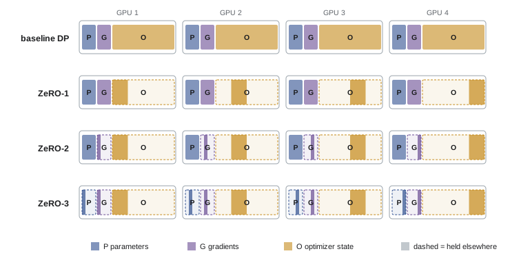
Rajbhandari and colleagues defined three progressively more aggressive stages, each partitioning another part of the model state across the \(N\) data-parallel devices. Writing \(\Psi\) for the parameter count and \(K = 12\) bytes per parameter for the FP32 master weights and Adam moments:
- Stage 1, optimizer state partitioning (\(P_{os}\)): each device keeps and updates the optimizer state for only \(1/N\) of the parameters. Memory per device becomes \(2\Psi + 2\Psi + K\Psi/N\).
- Stage 2, adding gradient partitioning (\(P_{os+g}\)): gradients are reduce-scattered rather than all-reduced, so each device receives only the summed gradients for the parameters it updates. Memory becomes \(2\Psi + (2 + K)\Psi/N\).
- Stage 3, adding parameter partitioning (\(P_{os+g+p}\)): each device stores only its shard of the BF16 parameters as well, gathering full layers temporarily when they are needed. Memory becomes \((4 + K)\Psi/N = 16\Psi/N\).
import numpy as np
# ZeRO memory per device (bytes) for psi parameters on N devices, K = 12 bytes of optimizer state
def zero_memory(psi, n, stage, k=12):
    p, g, o = 2 * psi, 2 * psi, k * psi
    if stage >= 1: o /= n
    if stage >= 2: g /= n
    if stage >= 3: p /= n
    return p + g + o
psi, n = 7.5e9, 64
for stage, name in enumerate(["baseline DP", "stage 1 (optimizer)", "stage 2 (+gradients)", "stage 3 (+parameters)"]):
    print(f"{name:22s}: {zero_memory(psi, n, stage)/1e9:6.1f} GB per GPU")
print("communication per step: stages 0-2 = 2 x params, stage 3 = 3 x params")
# Check that sharded training (stage 3 style) gives the same update as plain data parallelism
rng = np.random.default_rng(0)
dim, workers, lr = 12, 4, 0.1
w = rng.standard_normal(dim)
X = [rng.standard_normal((8, dim)) for _ in range(workers)]
y = [x @ np.ones(dim) for x in X]
def grad(w, x, t):
    return 2 * x.T @ (x @ w - t) / len(t)
# plain data parallel: every worker holds w, all-reduce the average gradient
g_avg = np.mean([grad(w, X[i], y[i]) for i in range(workers)], axis=0)
w_dp = w - lr * g_avg
# sharded: each worker owns one shard of w; all-gather before compute, reduce-scatter after
shards = np.array_split(w, workers)
full = np.concatenate(shards)                                   # all-gather
local = [grad(full, X[i], y[i]) for i in range(workers)]
summed = np.sum(local, axis=0) / workers
my_grad = np.array_split(summed, workers)                       # reduce-scatter
new_shards = [shards[i] - lr * my_grad[i] for i in range(workers)]
w_sharded = np.concatenate(new_shards)
print("sharded update equals data-parallel update:", np.allclose(w_dp, w_sharded))
print("parameter values stored per worker:", [s.size for s in new_shards], "of", dim)baseline DP : 120.0 GB per GPU stage 1 (optimizer) : 31.4 GB per GPU stage 2 (+gradients) : 16.6 GB per GPU stage 3 (+parameters) : 1.9 GB per GPU communication per step: stages 0-2 = 2 x params, stage 3 = 3 x params sharded update equals data-parallel update: True parameter values stored per worker: [3, 3, 3, 3] of 12
For the 7.5B model on 64 GPUs, the stages cut memory per GPU from 120 GB to about 31, 17 and 2 GB, reproducing the figures in the original paper. The numerical check confirms the essential point: sharding changes where data lives and how it moves, not the mathematics. The final model is identical to one trained with plain data parallelism.
How each stage communicates
Stages 1 and 2 cost no more communication than plain data parallelism. A standard all-reduce is a reduce-scatter followed by an all-gather (Lesson 6). With ZeRO stage 2, the reduce-scatter delivers each device the summed gradient for its shard; the device updates its shard of the parameters; and an all-gather distributes the updated parameters to all devices. The total, about \(2\Psi\) values per device per step, matches an all-reduce. Stage 3 adds traffic: parameters must be all-gathered before each layer's forward pass and again before its backward pass, because the full layer is discarded after use, and gradients are reduce-scattered. That totals about \(3\Psi\) values per device per step, 1.5 times plain data parallelism.
| Configuration | Memory per device | Communication per step | When to use |
|---|---|---|---|
| Data parallelism | 16Ψ | 2Ψ (all-reduce) | Model state fits easily on each device |
| ZeRO-1 | 4Ψ + 12Ψ/N | 2Ψ | Optimizer state is the main problem |
| ZeRO-2 | 2Ψ + 14Ψ/N | 2Ψ | Parameters fit, but gradients and optimizer do not |
| ZeRO-3 / FSDP full sharding | 16Ψ/N | 3Ψ | Even parameters do not fit on one device |
Fully Sharded Data Parallel in PyTorch
PyTorch FSDP, released in 2022 and described by Zhao and colleagues in 2023, implements stage-3-style sharding with practical refinements. The model is divided into units, typically one transformer block each. Each unit's parameters are flattened and sharded across devices. During the forward pass, FSDP all-gathers a unit's parameters just before it runs, computes, and frees the gathered copy; during the backward pass it gathers again, computes gradients, reduce-scatters them, and frees the full parameters. The optimizer then updates only the local shard. The second generation, FSDP2, shards each parameter individually along its first dimension using PyTorch's distributed tensor (DTensor) abstraction, simplifying interaction with other parallelism and with mixed precision.
Several mechanisms hide the extra communication. Prefetching starts the all-gather for the next unit while the current one computes; in the backward pass, FSDP can prefetch the previous unit's parameters. Communication runs on separate CUDA streams so it overlaps with computation. The size of each unit matters: larger units mean fewer, larger collectives that use bandwidth well but need more memory for the gathered parameters, while smaller units save memory but increase latency overhead. Mixed-precision settings let parameters be gathered in BF16 and gradients reduced in BF16 or FP32, while the sharded master weights stay in FP32.
Worked problem
Can communication be hidden?
A 13B model is trained with full sharding on 64 GPUs. Each GPU processes 16,384 tokens per step at a sustained 400 TFLOP/s, and the effective all-gather and reduce-scatter bandwidth per GPU is 40 GB/s. Is the step compute-bound or communication-bound?
Show solution
- Compute per GPU: \(6 \times 13 \times 10^9 \times 16{,}384 = 1.28 \times 10^{15}\) FLOPs, taking \(1.28 \times 10^{15} / 4 \times 10^{14} \approx 3.2\) s.
- Communication per GPU: about \(3\Psi\) BF16 values = \(3 \times 13 \times 10^9 \times 2 = 78\) GB.
- Communication time: \(78 / 40 \approx 1.95\) s.
- Communication (1.95 s) is shorter than compute (3.2 s), so with good prefetching it can be hidden.
Answer: Compute takes about 3.2 s and communication about 2 s, so the step can stay compute-bound if overlap works well; halving tokens per GPU would make communication exposed.
The example shows a general rule: sharded data parallelism is efficient when each device processes enough tokens per step that computation outlasts communication. Because computation per device falls as devices are added for a fixed global batch, while stage-3 communication per device stays at \(3\Psi\), there is a limit to how far full sharding alone scales.
Hybrid sharding
On large clusters, sharding across every device has two drawbacks: collectives span slower inter-server links, and latency grows with group size. Hybrid sharded data parallelism (HSDP in PyTorch, or ZeRO++ hierarchical partitioning in DeepSpeed) shards the model within a smaller group, often the eight GPUs of a server joined by NVLink or a few servers, and replicates that sharded group across the rest of the cluster with ordinary data parallelism. Parameter gathers then use the fast local links, and only gradient synchronization between replicas crosses the wider network. The trade-off is memory: each device holds \(1/8\) of the model state rather than \(1/N\). Other refinements reduce traffic further, such as quantizing parameters to 8 bits for the all-gather and gradients to 4 bits for the reduce-scatter in ZeRO++.
Offloading and ZeRO-Infinity
When even sharded state does not fit, ZeRO can offload it. ZeRO-Offload keeps optimizer state and the optimizer step on the CPU, transferring gradients down and updated parameters up each step. ZeRO-Infinity extends offloading to NVMe storage for parameters, gradients and optimizer state, with careful prefetching, and demonstrated fine-tuning of models with over a trillion parameters on a single server, slowly. These techniques make large models accessible on modest hardware, but for pre-training at scale, where throughput matters most, the state is normally kept in accelerator memory and sharded across enough devices.
Sharding in other frameworks
The same ideas appear in other systems under different names. In JAX, the GSPMD compiler partitions arrays across a mesh of devices according to sharding annotations: annotating parameters and optimizer state as sharded along a data axis produces the equivalent of ZeRO-3, and the compiler inserts the all-gathers and reduce-scatters automatically. Megatron-LM offers a distributed optimizer equivalent to ZeRO-1. Choosing between these systems is mostly a question of the framework a team uses; the memory and communication arithmetic is the same.
Choosing a configuration
A practical procedure for a new training job is: compute the model state at 16 bytes per parameter and the activations for the planned micro-batch; if they fit with plain data parallelism, use it, since it is simplest; otherwise try ZeRO-1 or ZeRO-2, which cost no extra communication; move to full sharding if parameters themselves do not fit; use hybrid sharding on large clusters to keep gathers on fast links; and when tokens per device become too few to hide stage-3 communication, or individual layers are too large for one device, add tensor and pipeline parallelism (Lessons 8 and 9). Profiling a few steps to measure exposed communication, rather than relying on calculation alone, confirms the choice.
Sharding and checkpoints
Sharding changes how checkpoints work. With full sharding, no single device holds the complete model, so each rank saves its own shard, and the checkpoint is a collection of files plus metadata describing how they fit together. Distributed checkpoint libraries can save in this sharded form and load into a different number of devices or a different parallel layout by redistributing the pieces, which is essential when a job is restarted on a different allocation or when a trained model is handed to an inference system with its own layout. Exporting a consolidated checkpoint, with full tensors gathered into standard files, is usually done separately at the end of training or for evaluation.
Debugging sharded training
Sharded training adds new failure modes. A rank that skips a collective, for example because a conditional branch in the model depends on its data, leaves the others waiting forever. Parameters that are accessed outside the framework's sharding units may be used while still sharded, producing shape errors or, worse, silently wrong results. Tools that log the sequence of collectives on each rank, and comparing a small sharded run against an unsharded run on the same data, help locate such problems. Starting with a configuration known to work and changing one setting at a time is the most reliable way to adopt sharding in a new codebase.
Common mistakes
MistakeUsing full sharding when model state fits.
InsteadPrefer plain DP or ZeRO-1/2, which add no communication.
MistakeAssuming sharding changes the trained model.
InsteadSharding gives identical updates to data parallelism.
MistakeSharding across all devices of a huge cluster.
InsteadUse hybrid sharding within fast-link groups.
MistakeIgnoring tokens per device.
InsteadKeep enough compute per step to hide gathers.
MistakeDisabling prefetching to save memory without measuring.
InsteadProfile exposed communication before changing overlap settings.
Summary and key terms
- Plain data parallelism stores redundant copies of the model state.
- ZeRO-1 shards optimizer state; ZeRO-2 adds gradients; ZeRO-3 adds parameters.
- Full sharding reduces memory per device to 16Ψ/N.
- ZeRO-1 and ZeRO-2 communicate as much as DP; ZeRO-3 about 1.5 times as much.
- FSDP gathers parameters per unit just in time and prefetches the next unit.
- Hybrid sharding keeps gathers on fast local links.
- Offloading to CPU or NVMe trades speed for capacity.
- ZeRO
- Zero Redundancy Optimizer, sharding model state.
- FSDP
- PyTorch Fully Sharded Data Parallel.
- Shard
- The portion of a tensor held by one device.
- Optimizer state partitioning
- ZeRO stage 1.
- Gradient partitioning
- ZeRO stage 2.
- Parameter partitioning
- ZeRO stage 3.
- FSDP unit
- Group of parameters gathered together.
- Prefetching
- Starting the next gather before it is needed.
- HSDP
- Hybrid sharding within groups, replication across them.
- ZeRO-Infinity
- Offloading model state to CPU and NVMe.
Practice problems
Work each problem on paper first, then reveal the answer to check.
Memory per GPU for a 20B model with full sharding on 32 GPUs?
Show answer
16 × 20 × 10⁹ / 32 = 10 GB.
Memory per GPU for the same model with ZeRO-1?
Show answer
4 × 20 + 12 × 20/32 = 87.5 GB.
Why does ZeRO-2 cost no extra communication?
Show answer
Reduce-scatter plus all-gather equals an all-reduce.
Why does ZeRO-3 communicate 3Ψ?
Show answer
Gathers in forward and backward plus a reduce-scatter.
What does FSDP free after a unit's forward pass?
Show answer
The gathered full parameters.
What does prefetching hide?
Show answer
All-gather latency for the next unit.
Trade-off of larger FSDP units?
Show answer
Better bandwidth use but more memory.
Why use hybrid sharding?
Show answer
Gathers stay on fast intra-node links.
What does ZeRO-Offload run on the CPU?
Show answer
The optimizer step and state.
How does JAX express sharding?
Show answer
Sharding annotations compiled by GSPMD.
Lesson quiz · 5 questions
Score 60% or more to complete this lesson.
Create a free account to save your progress, take quizzes and earn a certificate.