
AI-480 · Lesson 11 of 12 · 25 min
Reliability, profiling and efficiency at scale
A training run on thousands of accelerators for weeks or months is as much an operations challenge as a computational one. Components fail every few hours, slow devices hold back everyone else, numerical problems appear without warning, and small inefficiencies multiply across the whole cluster. The difference between a well-run and a poorly run job of the same size can be tens of percent of the total compute, which on a large run means millions of dollars and weeks of calendar time. This lesson covers the failure modes of large clusters, checkpointing strategy and the Young–Daly interval, fast recovery and elastic training, detecting stragglers and silent data corruption, profiling a training step, and the measures of efficiency, MFU and goodput, used to track a run.
Failure is routine at scale
Every component in a cluster has a small failure rate, but a cluster has a very large number of components. If each GPU, together with its share of the server, network and power, fails on average once every 50,000 hours, then a job using 16,384 GPUs experiences a failure about every three hours, and a job using 100,000 GPUs about every half hour. Meta's report on training Llama 3 405B gives a real example: during a 54-day period on 16,384 H100 GPUs, the job saw 466 interruptions, 419 of them unexpected, about one every three hours, and roughly 78 % of the unexpected ones were attributed to confirmed or suspected hardware problems, with faulty GPUs and their HBM memory the largest categories. Other causes included network switches and cables, host machines, software bugs and file system problems. Despite this, the team reported more than 90 % effective training time, thanks to automation.
Because synchronous training needs every worker, almost any failure stops the whole job. Recovery then means detecting the failure, replacing or excluding the faulty node, restarting all processes, loading the latest checkpoint and redoing the work lost since that checkpoint.
How often to checkpoint
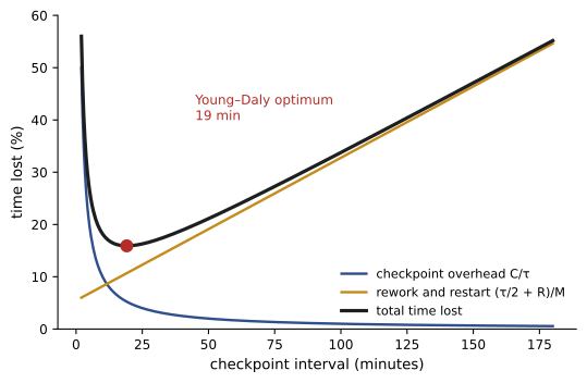
Checkpointing too rarely loses a lot of work at each failure; checkpointing too often spends too much time writing checkpoints. If writing a checkpoint takes time \(C\) and the mean time between failures is \(M\), the interval \(\tau\) that minimizes lost time is approximately the Young–Daly formula:
With this interval, the fraction of time lost is roughly \(C/\tau + (\tau/2 + R)/M\), where \(R\) is the restart time: the first term is checkpoint overhead and the second is the expected rework of half an interval plus the restart at each failure. Lowering \(C\) through asynchronous, sharded checkpoints, and lowering \(R\) through fast restarts, both reduce losses directly.
import numpy as np
# Cluster failure rate grows with size: MTBF_cluster = MTBF_component / N
gpu_mtbf_h = 50000.0                        # assumed hours between failures for one GPU and its share of the server
for n in (1024, 16384, 100000):
    print(f"{n:6d} GPUs: expected time between job interruptions {gpu_mtbf_h/n*60:6.0f} min")
# Young/Daly optimal checkpoint interval and the resulting overhead
def overhead(interval, ckpt, restart, mtbf):
    # fraction of time lost: checkpoint cost per interval + expected rework and restart per failure
    return ckpt / interval + (interval / 2 + restart) / mtbf
n = 16384; mtbf = gpu_mtbf_h / n * 3600      # seconds
ckpt, restart = 60.0, 600.0                  # seconds to write a checkpoint, seconds to restart
tau = np.sqrt(2 * ckpt * mtbf)
print(f"cluster MTBF {mtbf/3600:.2f} h; Young/Daly interval {tau/60:.1f} min")
for interval in (5 * 60, tau, 60 * 60, 3 * 3600):
    print(f"checkpoint every {interval/60:6.1f} min: time lost {overhead(interval, ckpt, restart, mtbf):5.1%}")
# Monte Carlo check of goodput over a 30-day run
rng = np.random.default_rng(0)
def goodput(interval, days=30, trials=200):
    total = days * 86400; useful = []
    for _ in range(trials):
        t = 0.0; done = 0.0
        while True:
            fail = rng.exponential(mtbf)
            if t + fail >= total:
                done += np.floor((total - t) / (interval + ckpt)) * interval
                break
            done += np.floor(fail / (interval + ckpt)) * interval   # work since the last checkpoint is lost
            t += fail + restart
        useful.append(done / total)
    return np.mean(useful)
print(f"simulated goodput, 30 days, Young/Daly interval: {goodput(tau):.1%}; hourly checkpoints: {goodput(3600):.1%}")
restart = 120.0
print(f"with restarts cut to 2 minutes: {goodput(tau):.1%}")1024 GPUs: expected time between job interruptions 2930 min 16384 GPUs: expected time between job interruptions 183 min 100000 GPUs: expected time between job interruptions 30 min cluster MTBF 3.05 h; Young/Daly interval 19.1 min checkpoint every 5.0 min: time lost 26.8% checkpoint every 19.1 min: time lost 15.9% checkpoint every 60.0 min: time lost 23.5% checkpoint every 180.0 min: time lost 55.2% simulated goodput, 30 days, Young/Daly interval: 85.2%; hourly checkpoints: 78.5% with restarts cut to 2 minutes: 88.9%
For 16,384 GPUs with a 60-second checkpoint and a 10-minute restart, the optimal interval is about 19 minutes, and about 16 % of the time is still lost. Checkpointing hourly loses 23 %, and every three hours loses more than half. Cutting the restart time to 2 minutes raises the simulated goodput from 85 % to 89 %, showing why large teams invest heavily in fast recovery.
Fast recovery and elastic training
Techniques that shorten recovery include keeping spare nodes ready so a failed node can be swapped without waiting for repair; holding recent checkpoints in host memory or on peer nodes, so a restart need not read from the file system; restarting only the affected processes where the framework allows; caching compiled kernels and communication setups to speed start-up; and automated health checks that run before nodes rejoin. Elastic training goes further, allowing a job to continue with fewer workers, for example by reducing the data-parallel degree and adjusting gradient accumulation to keep the global batch constant, then growing again when nodes return. Some systems keep redundant copies of optimizer state shards on other nodes so that work can resume without reloading a checkpoint at all.
Stragglers and hangs
Not all problems are clean failures. A straggler is a worker that runs slower than the others, perhaps because a GPU is throttling under heat or power limits, a network link has degraded to a lower speed, a host is busy with other processes, or a data loader is waiting on storage. Since synchronous steps wait for the slowest worker, one straggler slows the whole job. Hangs are worse: a worker stuck in a collective operation, perhaps because a peer crashed or a message was lost, can freeze thousands of others until a timeout fires. Practices include recording per-rank step times and collective durations to identify outliers, running communication libraries with watchdog timers that dump diagnostic information on hangs, testing nodes with burn-in workloads before admitting them, and automatically draining nodes whose performance falls below a threshold.
Silent data corruption
The most insidious failures produce wrong results without any error. Silent data corruption (SDC) occurs when a chip computes an incorrect value, through a manufacturing defect, aging or a transient fault, without raising an error. Google and Meta have both reported that a small fraction of processors in large fleets exhibit such faults. In training, a corrupted value can cause a loss spike or a NaN, or, more dangerously, slowly degrade the model. Defenses include memory protected by error-correcting codes (ECC), which catches most memory errors; periodic tests of each accelerator against known results; comparing gradient norms or checksums across data-parallel replicas, which should see consistent statistics; and monitoring the loss and gradient norms for anomalies, with the ability to roll back to an earlier checkpoint and exclude suspect hardware.
Profiling a training step
Improving efficiency starts with measurement. Profilers such as the PyTorch profiler and NVIDIA Nsight Systems record a timeline of every kernel, memory copy and collective on each GPU and every operation on the CPU. Reading the timeline of a step reveals where time goes:
- Compute kernels: matrix multiplications, attention and elementwise operations; their achieved FLOP/s and memory bandwidth show whether each is near its roofline (Lesson 2).
- Exposed communication: collectives that run while no computation overlaps them; ideally most communication is hidden.
- Pipeline bubbles: idle periods at the start and end of a step in pipeline-parallel jobs (Lesson 9).
- Host overhead: gaps between kernels when the CPU cannot launch work fast enough, often fixed by larger kernels, CUDA graphs or compilation.
- Data loading and synchronization: waits for input batches or for other ranks.
A common first step is a step-time breakdown into these categories, then targeting the largest. Optimizations follow from earlier lessons: fusing kernels, choosing better parallel configurations, increasing micro-batch size where memory allows, overlapping communication, and using lower precision.
Worked problem
Diagnosing low MFU
A 70B model is trained on 1,024 H100s (989 TFLOP/s peak) at 2.0 million tokens per step, with a step time of 3.6 s. A profile shows 2.3 s of compute kernels, 0.5 s of exposed data-parallel communication, 0.6 s of pipeline bubble and 0.2 s of host gaps. Calculate MFU and identify the best target for improvement.
Show solution
- Useful FLOPs per step: \(6 \times 70 \times 10^9 \times 2 \times 10^6 = 8.4 \times 10^{17}\).
- Achieved rate: \(8.4 \times 10^{17} / 3.6 = 2.33 \times 10^{17}\) FLOP/s.
- Peak: \(1024 \times 9.89 \times 10^{14} = 1.01 \times 10^{18}\) FLOP/s, so MFU ≈ 23 %.
- Non-compute time is 1.3 s: the pipeline bubble (0.6 s) is the largest, followed by exposed communication (0.5 s).
- Interleaving or more micro-batches could halve the bubble; better overlap could hide most of the communication.
Answer: MFU is about 23 %. Reducing the bubble and hiding communication could cut the step to about 2.6 s, raising MFU to about 32 %; the compute kernels themselves (about 36 % MFU on their own) could then be examined.
Measuring efficiency: MFU and goodput
MFU (Lesson 1) measures how well the hardware is used while the job is running. Goodput measures how much useful progress the job makes over wall-clock time, accounting for everything that does not advance training: failures, restarts, rework after rolling back to a checkpoint, time spent checkpointing, and time waiting for resources. Overall efficiency is roughly their product:
A run with 45 % MFU and 90 % goodput uses about 40 % of the cluster's theoretical capacity for useful training. Tracking both over the life of a run, alongside the loss curve, gradient norms and per-rank health metrics, is the core of large-scale training operations.
| Source of lost time | Typical remedy |
|---|---|
| Kernels below roofline | Fusion, better kernels, FlashAttention, larger matrices |
| Exposed communication | Overlap, bucketing, better parallel layout, faster links |
| Pipeline bubble | More micro-batches, interleaving, zero-bubble schedules |
| Recomputation | Selective rather than full activation checkpointing |
| Failures and restarts | Optimal checkpoint interval, fast recovery, spare nodes |
| Stragglers and hangs | Per-rank monitoring, watchdogs, node draining |
Reproducibility and run management
Large runs need to be reproducible enough to debug. Recording the exact code version, configuration, data order, random seeds and library versions with every checkpoint lets engineers resume and investigate. Full bitwise determinism is often impractical, because parallel reductions add numbers in varying order and some fast kernels are non-deterministic, but runs should be statistically reproducible: restarting from a checkpoint should give a matching loss curve. Teams typically run small-scale versions of every change first, use automated alerts on the loss and hardware metrics, and keep a log of every intervention, such as skipped data, learning-rate changes and hardware exclusions.
Learning from each run
Large training runs generate valuable operational knowledge. Teams that keep structured records of every failure, its cause, how long recovery took and how it was detected can improve their automation over time, identify unreliable hardware batches, and give realistic goodput estimates for future plans. Several organizations have published such records, which have become an important source of practical knowledge for the field.
Common mistakes
MistakeAssuming failures are rare.
InsteadPlan for interruptions every few hours at large scale.
MistakeCheckpointing on a fixed, arbitrary schedule.
InsteadUse the Young–Daly interval and reduce checkpoint cost.
MistakeIgnoring slow workers that do not crash.
InsteadMonitor per-rank timing and drain stragglers.
MistakeTrusting hardware outputs blindly.
InsteadTest for silent data corruption and monitor anomalies.
MistakeOptimizing without a profile.
InsteadBreak down step time and target the largest loss.
Summary and key terms
- Cluster failure rates grow with size; interruptions every few hours are normal.
- The Young–Daly interval √(2CM) balances checkpoint cost and lost work.
- Fast recovery, spare nodes and elastic training raise goodput.
- Stragglers and hangs slow or freeze synchronous jobs.
- Silent data corruption needs active testing and monitoring.
- Profiling breaks a step into compute, communication, bubbles and overhead.
- Effective efficiency is roughly MFU times goodput.
- MTBF
- Mean time between failures.
- Young–Daly interval
- Optimal checkpoint interval √(2CM).
- Goodput
- Useful training progress over wall-clock time.
- Elastic training
- Continuing with a changing number of workers.
- Straggler
- Worker slower than the others.
- Watchdog
- Timer that detects hangs.
- Silent data corruption
- Wrong results produced without an error.
- ECC
- Error-correcting code protecting memory.
- Step-time breakdown
- Division of step time into categories.
- Exposed communication
- Communication not overlapped with compute.
Practice problems
Work each problem on paper first, then reveal the answer to check.
Cluster MTBF for 8,192 GPUs at 40,000 h each?
Show answer
About 4.9 hours.
Young–Daly interval for C = 30 s and M = 4 h?
Show answer
√(2 × 30 × 14,400) ≈ 930 s ≈ 15.5 min.
Name two ways to reduce checkpoint cost.
Show answer
Asynchronous and sharded checkpoints, in-memory copies.
What does elastic training adjust to keep the global batch?
Show answer
Gradient accumulation steps.
Give two causes of stragglers.
Show answer
Thermal throttling, degraded links, busy hosts, slow data loading.
Why is silent data corruption dangerous?
Show answer
It produces wrong values with no error.
What is exposed communication?
Show answer
Communication not hidden behind computation.
MFU for 6 × 10¹⁷ useful FLOP/s on 2,048 GPUs of 989 TFLOP/s?
Show answer
About 30 %.
Effective efficiency at 40 % MFU and 85 % goodput?
Show answer
34 %.
Why is bitwise determinism hard?
Show answer
Parallel reductions vary in order; some kernels are non-deterministic.
Lesson quiz · 5 questions
Score 60% or more to complete this lesson.
Create a free account to save your progress, take quizzes and earn a certificate.