
AI-480 · Lesson 4 of 12 · 24 min
Numerical precision and mixed-precision training
Scientific computing traditionally uses 64-bit double precision, and early neural networks were trained in 32-bit single precision. Modern AI training runs mostly in 16-bit and increasingly 8-bit formats, and inference goes lower still, to 4-bit weights. Halving the number of bits per value roughly doubles arithmetic throughput on tensor cores, halves memory traffic and storage, and halves the data sent over the network, so precision is one of the most powerful levers on training cost. The challenge is that fewer bits mean less range and less accuracy, and naive low-precision training can diverge or silently lose information. This lesson explains how floating-point formats work, the formats used in AI, mixed-precision training with master weights and loss scaling, FP8 training with scaling factors, quantization for inference, and the numerical safeguards that keep large runs stable.
How floating-point numbers work
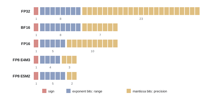
A binary floating-point number has a sign bit, an exponent and a mantissa (also called the significand). Its value is approximately \((-1)^s \times 1.m \times 2^{e - \text{bias}}\). The exponent bits set the range: how large and how small a number can be represented. The mantissa bits set the precision: how finely numbers are spaced. With \(p\) mantissa bits, the gap between 1 and the next representable number, the machine epsilon, is \(2^{-p}\), so relative rounding error is at most about \(2^{-(p+1)}\). Numbers too large overflow to infinity; numbers too small underflow to subnormal values with reduced precision and eventually to zero.
Formats used in AI
| Format | Sign / exponent / mantissa bits | Largest value | Machine epsilon | Typical use |
|---|---|---|---|---|
| FP32 | 1 / 8 / 23 | 3.4 × 10³⁸ | 1.2 × 10⁻⁷ | Master weights, optimizer state, accumulation |
| TF32 | 1 / 8 / 10 | 3.4 × 10³⁸ | 9.8 × 10⁻⁴ | Tensor-core matmuls from FP32 inputs |
| FP16 | 1 / 5 / 10 | 65,504 | 9.8 × 10⁻⁴ | Mixed-precision training with loss scaling, inference |
| BF16 | 1 / 8 / 7 | 3.4 × 10³⁸ | 7.8 × 10⁻³ | Default training format on modern accelerators |
| FP8 E4M3 | 1 / 4 / 3 | 448 | 0.125 | Forward-pass weights and activations |
| FP8 E5M2 | 1 / 5 / 2 | 57,344 | 0.25 | Gradients, which need more range |
| INT8, INT4 | Integers with a scale factor | Set by scale | Uniform steps | Quantized inference |
BF16, the "brain floating point" format developed at Google Brain, keeps FP32's 8 exponent bits and simply drops 16 mantissa bits. It has the same range as FP32, so values rarely overflow or underflow, but only about two to three significant decimal digits. FP16 has three more mantissa bits and thus finer precision, but a much narrower range: its largest value is 65,504 and its smallest normal value is about \(6.1 \times 10^{-5}\). Neural network training turns out to tolerate low precision in individual values remarkably well but to be sensitive to range, which is why BF16 became the default.
import numpy as np
# Emulate BF16 by keeping the top 16 bits of an FP32 value (round to nearest even)
def to_bf16(x):
    x = np.asarray(x, dtype=np.float32)
    bits = x.view(np.uint32).astype(np.uint64)
    rounding = ((bits >> 16) & 1) + 0x7FFF
    return ((bits + rounding) >> 16 << 16).astype(np.uint32).view(np.float32)
vals = np.array([3.14159265, 1000.1, 70000.0, 1e-6, 1e-9], dtype=np.float32)
with np.errstate(over="ignore"):
    fp16 = vals.astype(np.float16)
for v, h, b in zip(vals, fp16, to_bf16(vals)):
    print(f"fp32={v:<12.6g} fp16={float(h):<12.6g} bf16={float(b):<12.6g}")
print("machine epsilon  fp16:", np.finfo(np.float16).eps, " bf16: 2**-7 =", 2.0**-7, " fp32:", np.finfo(np.float32).eps)
# Gradient underflow in FP16 and the effect of loss scaling
rng = np.random.default_rng(1)
grads = (rng.standard_normal(100000) * 1e-7).astype(np.float32)
lost = np.mean(grads.astype(np.float16) == 0)
scale = 2.0**16
scaled = (grads * scale).astype(np.float16)
recovered = scaled.astype(np.float32) / scale
print(f"fraction of gradients flushed to zero in fp16: {lost:.1%}")
print(f"with loss scale 2**16: zeros={np.mean(scaled == 0):.1%}, mean relative error={np.mean(np.abs(recovered - grads) / np.abs(grads)):.2%}")
# Accumulating many small updates: why master weights stay in FP32
w16 = np.float16(1.0); w32 = np.float32(1.0)
for _ in range(10000):
    w16 = np.float16(w16 + np.float16(1e-4)); w32 = np.float32(w32 + np.float32(1e-4))
print(f"1.0 + 10,000 updates of 1e-4: fp16 weight={float(w16):.4f}, fp32 weight={float(w32):.4f}, exact=2.0000")fp32=3.14159 fp16=3.14062 bf16=3.14062 fp32=1000.1 fp16=1000 bf16=1000 fp32=70000 fp16=inf bf16=70144 fp32=1e-06 fp16=1.01328e-06 bf16=9.98378e-07 fp32=1e-09 fp16=0 bf16=9.96806e-10 machine epsilon fp16: 0.000977 bf16: 2**-7 = 0.0078125 fp32: 1.1920929e-07 fraction of gradients flushed to zero in fp16: 23.5% with loss scale 2**16: zeros=0.0%, mean relative error=0.02% 1.0 + 10,000 updates of 1e-4: fp16 weight=1.0000, fp32 weight=2.0002, exact=2.0000
The output illustrates three facts. FP16 overflows at 70,000 while BF16 represents it, coarsely; FP16 flushes a value of \(10^{-9}\) to zero while BF16 keeps it. Without scaling, nearly a quarter of a set of small gradients vanish in FP16, but multiplying them by \(2^{16}\) first preserves them all. And adding 10,000 updates of \(10^{-4}\) to a weight of 1.0 in FP16 achieves nothing, because each update is smaller than half the gap between 1.0 and the next FP16 number, so every addition rounds back to 1.0. This last effect, called swamping, is why weights are kept in FP32.
Mixed-precision training
Mixed-precision training, described by Micikevicius and colleagues at NVIDIA and Baidu in 2018, performs the expensive matrix multiplications in 16-bit precision while protecting the parts of training that need more. Its main elements are:
- FP32 master weights: the optimizer keeps an FP32 copy of every weight and applies updates to it; a 16-bit copy is made for the forward and backward passes.
- FP32 accumulation: tensor cores multiply 16-bit inputs but accumulate sums in FP32, so long dot products do not lose precision.
- Loss scaling (for FP16): the loss is multiplied by a large factor before backpropagation, shifting small gradients into FP16's representable range; gradients are divided by the same factor before the update.
- Selected operations in FP32: reductions such as softmax normalization, layer normalization statistics and the loss itself are often computed in FP32.
Dynamic loss scaling chooses the factor automatically: start large, for example \(2^{16}\); if any gradient overflows to infinity or NaN, skip that step and halve the scale; after a run of successful steps, double it. With BF16, gradients rarely underflow, so loss scaling is usually unnecessary, which simplifies training considerably. Frameworks implement all of this as automatic mixed precision (AMP), for example torch.autocast in PyTorch.
Mixed precision therefore does not reduce optimizer memory; it actually adds the 16-bit copies. Its benefits are faster arithmetic, smaller activations and less communication. Lesson 7 shows how sharding attacks the 16 bytes per parameter.
FP8 training
Hopper-generation GPUs added FP8 tensor cores with twice the throughput of BF16. FP8 has so few bits that a single fixed format cannot cover the range of values in a network, so FP8 training relies on scaling factors: each tensor, or each block of a tensor, is multiplied by a scale chosen so that its largest values fit just within the format's range, then the result is cast to FP8. NVIDIA's Transformer Engine library uses per-tensor scaling with "delayed scaling", estimating each scale from the maximum absolute values observed in recent steps. Typically E4M3 is used for weights and activations in the forward pass and E5M2, with its wider range, for gradients.
Finer-grained scaling improves accuracy further. DeepSeek-V3, a 671-billion-parameter mixture-of-experts model released at the end of 2024, was trained largely in FP8 using scales for small tiles of activations (1 × 128) and blocks of weights (128 × 128), with higher-precision accumulation, and its authors reported loss within a fraction of a percent of a BF16 baseline. Blackwell GPUs support microscaling formats, such as MXFP8 and MXFP4 defined by the Open Compute Project, in which every block of 32 values shares an 8-bit scale, making fine-grained scaling a hardware feature.
Quantization for inference
Inference can use even lower precision because the model is fixed and only needs to produce accurate outputs, not to learn. Quantization maps floating-point values to integers with a scale (and sometimes a zero point):
Common approaches include INT8 quantization of weights and activations; weight-only INT4 or FP4 quantization for large language models, where memory bandwidth during decoding is the bottleneck, using methods such as GPTQ and AWQ that minimize the error on calibration data; and quantizing the key-value cache that stores attention state for long contexts. Quantization-aware training simulates quantization during training or fine-tuning so the model learns to tolerate it. Because small-batch decoding is memory-bound (Lesson 2), 4-bit weights can speed generation by nearly four times relative to 16-bit weights with only a small loss in quality for many models.
Worked problem
Quantizing a weight block
A block of weights has a maximum absolute value of 0.84. Quantize the weight 0.37 to symmetric INT8, and find the dequantized value and error.
Show solution
- Scale: \(s = 0.84 / 127 \approx 0.006614\).
- Quantized value: \(q = \operatorname{round}(0.37 / 0.006614) = \operatorname{round}(55.94) = 56\).
- Dequantized value: \(\hat{x} = 56 \times 0.006614 \approx 0.3704\).
- Error: \(0.3704 - 0.37 \approx 0.0004\), within half a step of 0.0033.
Answer: q = 56; the dequantized value is about 0.3704, an error of about 0.0004.
Keeping low-precision training stable
Large training runs occasionally suffer loss spikes or divergence, and low precision makes some causes worse. Standard safeguards include subtracting the maximum before exponentiating in softmax so exponentials cannot overflow; computing normalization statistics in FP32; gradient clipping to a maximum norm; careful initialization and learning-rate warm-up; techniques that limit the growth of attention logits, such as normalizing queries and keys; monitoring for NaN and infinite values and skipping bad steps; and keeping checkpoints so that a run can be rewound past a spike and resumed with different data order or a lower learning rate. Stochastic rounding, which rounds up or down at random with probability proportional to the distance, can prevent the swamping seen in the code example and is supported by some accelerators.
Choosing a precision recipe
In practice, teams choose from a small number of established recipes. The most common for large language model pre-training on recent GPUs and TPUs is BF16 mixed precision: BF16 weights, activations and gradients for computation, FP32 master weights and optimizer state, FP32 accumulation in matrix multiplications, and selected operations in FP32. Teams seeking more speed on Hopper or Blackwell GPUs add FP8 for the large matrix multiplications in transformer blocks, often keeping the first and last layers, attention softmax and normalization in higher precision, and validating with a smaller-scale run that the loss curve matches BF16 closely. FP16 with loss scaling remains in use on older hardware without BF16 support. Whatever the recipe, the essential test is empirical: train a smaller model with both the new and a trusted recipe and compare their loss curves and downstream evaluations before committing a large run.
Precision and communication
Precision choices affect communication as well as computation. Gradients reduced across data-parallel workers in BF16 halve network traffic compared with FP32, but summing many BF16 values loses precision, so some systems reduce in FP32 or use higher-precision accumulation inside the reduction. Parameters all-gathered in sharded training can be sent in BF16 or even FP8. Activations sent between pipeline stages and in tensor-parallel collectives can also be compressed. Each saving must be checked for its effect on convergence, since errors introduced in communication accumulate across thousands of steps.
Precision and optimizer state
The optimizer state itself can be stored in lower precision. Eight-bit Adam implementations store the two moments as 8-bit values with block-wise scales and dynamic quantization, cutting optimizer memory by about three quarters, and have been shown to match 32-bit Adam on many tasks. Some systems store master weights in BF16 with compensation terms that capture the rounding error, such as Kahan summation, which recovers most of the accuracy of FP32 master weights at lower memory cost. These techniques are especially attractive for fine-tuning on limited hardware.
Common mistakes
MistakeKeeping weights only in 16-bit precision.
InsteadKeep FP32 master weights so small updates are not lost.
MistakeTraining in FP16 without loss scaling.
InsteadUse dynamic loss scaling, or BF16.
MistakeCasting to FP8 without scaling factors.
InsteadScale per tensor or per block to fit the format's range.
MistakeAssuming mixed precision cuts optimizer memory.
InsteadIt still needs about 16 bytes per parameter with Adam.
MistakeQuantizing for inference without evaluation.
InsteadMeasure quality on representative tasks after quantization.
Summary and key terms
- Exponent bits set range; mantissa bits set precision.
- BF16 keeps FP32's range with less precision and is the default training format.
- FP16 needs loss scaling because small gradients underflow.
- Mixed precision uses 16-bit matmuls with FP32 accumulation and master weights.
- FP8 training uses E4M3 and E5M2 with per-tensor or per-block scaling.
- Quantization to INT8 or 4-bit formats speeds memory-bound inference.
- Stability safeguards include FP32 reductions, clipping and monitoring.
- Mantissa
- Bits that set a float's precision.
- Exponent
- Bits that set a float's range.
- Machine epsilon
- Gap between 1 and the next representable number.
- BF16
- Brain floating point: 8 exponent, 7 mantissa bits.
- Master weights
- FP32 copy of weights used for updates.
- Loss scaling
- Multiplying the loss to keep gradients representable.
- Swamping
- Small additions lost when rounding to a large value.
- Scaling factor
- Multiplier mapping values into a format's range.
- Quantization
- Mapping values to low-bit integers with a scale.
- Stochastic rounding
- Random rounding proportional to distance.
Practice problems
Work each problem on paper first, then reveal the answer to check.
Which part of a float sets its range?
Show answer
The exponent.
What is the largest FP16 value?
Show answer
65,504.
Why did BF16 replace FP16 for most training?
Show answer
It has FP32's range, so loss scaling is rarely needed.
What does dynamic loss scaling do after an overflow?
Show answer
Skips the step and halves the scale.
Why keep master weights in FP32?
Show answer
Small updates would be lost to rounding in 16-bit.
How many bytes per parameter does Adam need in mixed precision?
Show answer
About 16.
Which FP8 format suits gradients?
Show answer
E5M2, for its range.
Quantize 0.5 to INT8 if max |x| = 1.27.
Show answer
s = 0.01; q = 50.
Why does 4-bit weight quantization speed decoding?
Show answer
Decoding is memory-bound; fewer bytes are read.
Name two stability safeguards.
Show answer
Softmax max subtraction, FP32 norms, gradient clipping, warm-up.
Lesson quiz · 5 questions
Score 60% or more to complete this lesson.
Create a free account to save your progress, take quizzes and earn a certificate.