
AI-480 · Lesson 10 of 12 · 24 min
Clusters, interconnects and storage
A training cluster is far more than a collection of accelerators. The links inside each server, the network joining thousands of servers, the storage that feeds data and absorbs checkpoints, and the software that schedules jobs all shape how fast a model trains, and a weakness in any of them can idle the most expensive chips. The previous lessons treated communication as a bandwidth and a latency; this lesson looks at the physical systems behind those numbers. It covers server design and the NVLink scale-up domain, scale-out networks built on InfiniBand and Ethernet with remote direct memory access, network topologies and how parallelism maps onto them, congestion and reliability in the network, the storage systems used for training data and checkpoints, and cluster scheduling.
Inside the server
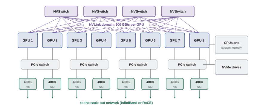
A typical AI training server, such as an NVIDIA DGX or HGX H100 system, holds eight GPUs on a baseboard, two host CPUs with a terabyte or more of memory, local NVMe drives and eight or more network adapters. The GPUs connect to each other through NVLink and NVSwitch chips, giving each GPU 900 GB/s of total bandwidth to any other GPU in the server, roughly 14 times a PCIe 5.0 x16 link. The GPUs connect to the CPUs, drives and network adapters through PCIe switches. A common design gives each GPU its own 400 Gb/s network adapter on the same PCIe switch, so GPU memory can be sent to the network without passing through the CPU, a capability called GPUDirect RDMA.
The group of accelerators joined by the fastest links is called the scale-up domain. For years it was a single eight-GPU server. Rack-scale systems such as the GB200 NVL72 extend NVLink to 72 GPUs across a rack using copper cable spines, and TPU pods join thousands of chips through their own inter-chip interconnect. Larger scale-up domains let tensor and expert parallelism (Lesson 8) span more devices, which is why they have become a focus of system design. Beyond the scale-up domain, the scale-out network takes over.
Scale-out networks and RDMA
Between servers, training clusters use networks designed for low latency and high bandwidth with minimal CPU involvement. Remote direct memory access (RDMA) lets a network adapter read from or write to memory on another machine without involving either machine's operating system on the data path, cutting latency to a few microseconds and freeing CPUs. Two families dominate:
- InfiniBand: a high-performance network technology long used in supercomputers, with credit-based flow control that avoids packet loss, built-in adaptive routing and in-network computing features such as NVIDIA's SHARP, which performs reductions inside switches. NDR InfiniBand runs at 400 Gb/s per port and XDR at 800 Gb/s.
- Ethernet with RoCE: RDMA over Converged Ethernet (RoCEv2) carries RDMA traffic over standard Ethernet and IP, using priority flow control and congestion notification to approximate a lossless network. Ethernet benefits from a broad vendor ecosystem, and the Ultra Ethernet Consortium, formed in 2023, is developing transport improvements for AI and high-performance computing.
Both are used at very large scale. Meta, for example, described two clusters of about 24,000 H100 GPUs in 2024, one built with RoCE and one with InfiniBand, and reported that both could be tuned to train large models effectively.
Topologies
The arrangement of switches and links, the topology, determines how much bandwidth is available between any two groups of devices. The most common topology for GPU clusters is the fat tree, a folded Clos network: servers connect to leaf switches, leaf switches connect to spine switches, and for very large clusters spines connect to a further core layer. A fat tree is non-blocking when each switch has as many links going up as coming down, so that any half of the endpoints can talk to the other half at full speed; the bandwidth across such a cut is called the bisection bandwidth. Building with switches of radix \(k\), a two-tier fat tree connects up to \(k^2/2\) endpoints and a three-tier fat tree up to \(k^3/4\).
import numpy as np
# Sizing a non-blocking fat-tree (folded Clos) network built from radix-k switches
def fat_tree(endpoints, k=64):
    half = k // 2
    if endpoints <= k:
        return 1, {"single switch": 1}
    if endpoints <= k * half:                         # two tiers: leaf and spine
        leaves = int(np.ceil(endpoints / half))
        spines = int(np.ceil(leaves * half / k))
        return 2, {"leaf": leaves, "spine": spines}
    pods = int(np.ceil(endpoints / (half * half)))  # three tiers
    leaves = pods * half; aggs = pods * half
    cores = int(np.ceil(aggs * half / k))
    return 3, {"leaf": leaves, "aggregation": aggs, "core": cores}
print(f"radix-64 capacity: two tiers {64*32} endpoints, three tiers {64**3//4}")
for gpus in (512, 2048, 16384, 65536):
    tiers, sw = fat_tree(gpus)
    total = sum(sw.values())
    print(f"{gpus:6d} GPU NICs: {tiers} tiers, switches {sw}, total {total}")
# Bisection bandwidth with one 400 Gb/s NIC per GPU
for gpus in (2048, 16384):
    print(f"{gpus} GPUs: full bisection bandwidth = {gpus/2*400/8/1000:.0f} TB/s")
# Checkpoint sizes and write times
for name, params in [("8B", 8e9), ("70B", 70e9), ("405B", 405e9)]:
    size = params * (2 + 12)                         # BF16 weights plus FP32 master and Adam moments
    for bw in (50e9, 1e12):
print(f"{name:4s} checkpoint {size/1e12:5.2f} TB at {bw/1e9:5.0f} GB/s aggregate: {size/bw:7.1f} s")radix-64 capacity: two tiers 2048 endpoints, three tiers 65536
512 GPU NICs: 2 tiers, switches {'leaf': 16, 'spine': 8}, total 24
2048 GPU NICs: 2 tiers, switches {'leaf': 64, 'spine': 32}, total 96
16384 GPU NICs: 3 tiers, switches {'leaf': 512, 'aggregation': 512, 'core': 256}, total 1280
65536 GPU NICs: 3 tiers, switches {'leaf': 2048, 'aggregation': 2048, 'core': 1024}, total 5120
2048 GPUs: full bisection bandwidth = 51 TB/s
16384 GPUs: full bisection bandwidth = 410 TB/s
8B checkpoint 0.11 TB at 50 GB/s aggregate: 2.2 s
8B checkpoint 0.11 TB at 1000 GB/s aggregate: 0.1 s
70B checkpoint 0.98 TB at 50 GB/s aggregate: 19.6 s
70B checkpoint 0.98 TB at 1000 GB/s aggregate: 1.0 s
405B checkpoint 5.67 TB at 50 GB/s aggregate: 113.4 s
405B checkpoint 5.67 TB at 1000 GB/s aggregate: 5.7 sWith 64-port switches, a two-tier network reaches 2,048 GPU network adapters and a three-tier network 65,536. A 16,384-GPU cluster needs 1,280 switches and tens of thousands of optical links, and its full bisection bandwidth exceeds 400 TB/s. Networks of this size are among the largest single-purpose networks ever built, and their cost is a substantial fraction of the cluster.
Many GPU clusters use a rail-optimized variant: the GPU in position 1 of every server connects to the same leaf switch, or rail, as do all GPUs in position 2, and so on. Collective operations among GPUs with the same position, the common pattern when tensor parallelism occupies each server and data or pipeline parallelism spans servers, then cross only one switch hop. TPU pods instead use torus topologies, in which each chip links directly to its neighbors in three dimensions, suiting the regular communication patterns compiled by XLA. Some designs deliberately oversubscribe the upper tiers, providing less bandwidth than a full fat tree, to save cost when traffic is mostly local.
Mapping parallelism to the network
Each parallelism dimension has a characteristic traffic pattern, and good configurations place each where the network serves it best:
- Tensor and expert parallelism: heavy, latency-sensitive collectives in every layer; place within the scale-up domain.
- Pipeline parallelism: point-to-point transfers between neighboring stages; place stages so neighbors are close, often on the same rail or leaf.
- Data parallelism and sharding: large all-reduces, reduce-scatters and all-gathers once per step or per layer; can span the whole cluster, using hierarchical algorithms and overlap.
Communication libraries such as NCCL detect the topology at start-up, building rings and trees that follow it, and schedulers try to allocate jobs to servers under as few switches as possible to keep traffic local.
| Link | Typical bandwidth per GPU | Latency | Used for |
|---|---|---|---|
| HBM (on package) | 3–8 TB/s | Hundreds of ns | Weights, activations, optimizer state |
| NVLink / NVSwitch | 900–1,800 GB/s | About 1 µs | Tensor, sequence and expert parallelism |
| PCIe 5.0 x16 | 64 GB/s each way | About 1 µs | Host memory, offloading, network adapters |
| InfiniBand or RoCE NIC | 50–100 GB/s (400–800 Gb/s) | A few µs | Data, pipeline and sharded parallelism |
| Parallel file system | Hundreds of GB/s to TB/s in aggregate | Milliseconds | Training data, checkpoints |
Congestion, routing and network reliability
Training traffic is unusually demanding for networks. Collective operations start on thousands of GPUs at the same instant and send large, synchronized bursts, so a few congested links can slow every worker. Traffic is dominated by a small number of very large flows, which defeats the hash-based load balancing used in conventional data center networks: two large flows hashed onto the same link run at half speed while other links sit idle. Remedies include adaptive routing, which steers packets onto less loaded paths; packet spraying, which spreads one flow across many paths and reorders packets at the destination; tuned congestion control; and scheduling collectives so that they do not collide. Network faults are also common at scale: optical transceivers and cables fail, links flap up and down, and a single bad link can cause hangs or timeouts in collective operations. Monitoring link error counters and quickly draining faulty components are routine operations.
Storage for training data
Training data for language models is usually pre-processed into tokenized shards: large files containing sequences of token IDs, often packed to the training sequence length, which can be read sequentially with little CPU work. Data for images, video and multimodal models is larger and needs decoding and augmentation, which can strain CPU resources. Data loaders run in background processes, prefetching and shuffling data ahead of the accelerators; the aim is that the accelerators never wait. Storage systems include parallel file systems such as Luster, IBM Storage Scale (GPFS), WEKA and VAST, which spread files across many servers for high aggregate bandwidth, and object stores such as Amazon S3 and Google Cloud Storage, often with a caching layer. Data pipelines must also be deterministic and resumable: after a restart, training should continue from the exact point in the data stream where it stopped, so that no data is skipped or repeated.
Worked problem
Is the data pipeline fast enough?
A cluster of 2,048 GPUs trains a language model at 3,000 tokens per second per GPU. Tokens are stored as 4-byte integers. What read bandwidth must storage sustain? How does this change for a video model reading 2 MB of compressed video per training sample at 2 samples per second per GPU?
Show solution
- Language model tokens per second: \(2048 \times 3000 = 6.1 \times 10^6\).
- Bytes per second: \(6.1 \times 10^6 \times 4 \approx 24.6\) MB/s, trivial for any parallel file system.
- Video model: \(2048 \times 2 \times 2\) MB = 8.2 GB/s of sustained reads, plus decoding work on the CPUs.
Answer: About 25 MB/s for text, easily served; about 8 GB/s for video, which needs a high-performance storage system and enough CPU or hardware decoders.
Checkpoint storage
Checkpoints are the other heavy storage workload. A full checkpoint includes model weights, optimizer state, the data loader position and random number generator states, so it is about 14 to 16 bytes per parameter: several terabytes for a model of a few hundred billion parameters. Writing it through a single node would take hours; instead, every rank writes its own shard in parallel, and the checkpoint's speed depends on the storage system's aggregate bandwidth. Asynchronous checkpointing copies the state from GPU memory to host memory quickly, lets training continue, and writes to storage in the background. Distributed checkpoint formats, such as PyTorch Distributed Checkpoint, also allow resharding, so a checkpoint saved with one parallel configuration can be loaded with another. Lesson 11 covers how often to checkpoint.
Scheduling and cluster software
Clusters are shared among many jobs and teams through schedulers. Slurm, widely used in high-performance computing, allocates whole servers to batch jobs and supports topology-aware placement; Kubernetes, common in cloud environments, schedules containers and is extended with operators for distributed training. Schedulers handle queueing and priorities, gang scheduling (starting all of a job's workers together or none at all), placement near each other in the network, preemption, and draining and replacing failed nodes. Around them sit health checks, monitoring of GPU, network and storage metrics, and logging that lets engineers trace problems across thousands of processes.
Common mistakes
MistakeTreating the cluster network as an afterthought.
InsteadDesign topology and bandwidth with the parallelism plan.
MistakeRunning tensor parallelism across the scale-out network.
InsteadKeep it within the NVLink scale-up domain.
MistakeRelying on hash-based load balancing for large flows.
InsteadUse adaptive routing or packet spraying.
MistakeWriting checkpoints from one node.
InsteadWrite sharded checkpoints in parallel, asynchronously.
MistakeUsing non-resumable data pipelines.
InsteadSave the data position so restarts neither skip nor repeat data.
Summary and key terms
- Servers join GPUs with NVLink and give each GPU its own network adapter.
- The scale-up domain is the group joined by the fastest links.
- RDMA over InfiniBand or RoCE provides low-latency scale-out networking.
- Fat trees provide full bisection bandwidth; rail-optimized designs suit GPU collectives.
- Parallelism dimensions are mapped onto the network by traffic intensity.
- Large synchronized flows need adaptive routing and careful congestion control.
- Storage must feed data continuously and absorb large parallel checkpoints.
- NVSwitch
- Switch chip joining GPUs over NVLink.
- Scale-up domain
- Accelerators joined by the fastest links.
- Scale-out network
- Network joining servers in a cluster.
- RDMA
- Remote direct memory access.
- GPUDirect RDMA
- Network access to GPU memory without the CPU.
- RoCE
- RDMA over Converged Ethernet.
- Fat tree
- Folded Clos network of leaf and spine switches.
- Bisection bandwidth
- Bandwidth across a cut halving the network.
- Rail-optimized
- Same-position GPUs share a leaf switch.
- Gang scheduling
- Starting all of a job's workers together.
Practice problems
Work each problem on paper first, then reveal the answer to check.
How much NVLink bandwidth does an H100 have?
Show answer
900 GB/s total.
What does GPUDirect RDMA avoid?
Show answer
Copying GPU data through host memory and CPU.
Name two scale-out network technologies.
Show answer
InfiniBand and RoCE Ethernet.
Maximum endpoints of a two-tier fat tree with 48-port switches?
Show answer
48²/2 = 1,152.
Bisection bandwidth for 4,096 GPUs at 400 Gb/s each?
Show answer
2,048 × 50 GB/s ≈ 102 TB/s.
What does a rail-optimized topology connect to one leaf?
Show answer
The same-position GPU from every server.
Why does hash-based load balancing struggle with training traffic?
Show answer
A few huge flows collide on the same links.
Read bandwidth for 1,024 GPUs at 4,000 tokens/s with 4-byte tokens?
Show answer
About 16 MB/s.
What does asynchronous checkpointing do?
Show answer
Copies state to host memory and writes in the background.
What is gang scheduling?
Show answer
Starting all workers of a job together.
Lesson quiz · 5 questions
Score 60% or more to complete this lesson.
Create a free account to save your progress, take quizzes and earn a certificate.