Reinforcement learning for control and sim-to-real transfer

Some robot skills are very hard to engineer by hand. Walking over rubble, recovering from a shove, spinning an object in the fingers, or catching a ball all involve complex contact dynamics that defy simple models and controllers. Reinforcement learning (RL) lets a robot learn such skills by trial and error, guided by a reward signal, and over the past decade it has produced some of the most striking results in robotics, especially in legged locomotion. Because trial and error on real hardware is slow, expensive and dangerous, most robot RL happens in simulation, and the central practical challenge is making policies trained in simulation work on real robots. This lesson covers the RL formulation for robots, model-free algorithms used in practice, massively parallel simulation, reward design, the sim-to-real gap and the techniques that close it, privileged teacher-student training, model-based RL, and the safety issues of learning on and deploying to real hardware.

The reinforcement learning formulation

RL frames control as a Markov decision process: at each time step the agent observes a state (or an observation of it), takes an action, receives a reward, and the environment moves to a new state. The goal is a policy, a mapping from observations to actions, that maximizes expected cumulative discounted reward. For robots:

• Observations typically include joint positions and velocities, IMU readings, previous actions, commands (such as desired velocity), and sometimes camera images or height maps of the terrain.
• Actions are often joint position targets for low-level PD controllers (Lesson 8), sometimes joint torques or end-effector targets.
• Rewards encode the task (track a velocity, reach a goal, keep an object in hand) plus regularization terms that penalize energy use, jerky motion, joint limit violations, falling and undesirable contacts.
• Episodes end on success, failure (falling over) or a time limit, and the environment is reset with randomized initial conditions.

Algorithms used in practice

Deep RL algorithms fall into two main families. On-policy methods such as Proximal Policy Optimization (PPO) collect fresh experience with the current policy, update it with clipped policy-gradient steps for stability, and discard the data. PPO is simple, robust and scales well to thousands of parallel simulated robots, which has made it the dominant choice for locomotion. Off-policy methods such as Soft Actor-Critic (SAC) store experience in a replay buffer and reuse it many times, making them far more sample-efficient, which matters when learning on real hardware or with expensive simulators; SAC also encourages exploration through an entropy bonus. Value-based methods such as Q-learning learn the value of each action, and the simplest tabular version illustrates key ideas, as in the example below.

Simulation at scale

Modern GPU-accelerated simulators, such as Isaac Lab, MuJoCo with GPU backends (MJX and MuJoCo Playground), Genesis and Brax, can run thousands of robot instances in parallel on a single GPU, generating years of simulated experience in hours. A quadruped walking policy that once took days to train can now be trained in minutes. Scale changes what is possible: policies can be trained across huge variations of terrain, friction, mass and sensor noise, and automatic curricula can increase difficulty as the policy improves, for example from flat ground to stairs and rubble.

Reward design

Rewards are the specification of what the robot should learn, and RL is notoriously good at finding unintended ways to maximize them, sometimes called reward hacking: a robot rewarded for forward velocity may learn to vibrate forward on its knees, or exploit a simulator bug that lets feet penetrate the ground. Good reward design combines a clear task term with penalties for undesirable behavior, keeps terms on comparable scales, and is checked by watching rollouts, not just reward curves. Shaping rewards (intermediate rewards that guide learning) can speed training but can also change what is optimal if poorly designed. Imitation of reference motions, such as motion-capture clips for natural humanoid gaits, provides another form of guidance (Lesson 10).

The sim-to-real gap

Simulated robots differ from real ones in many ways: inaccurate masses and inertias, simplified contact and friction models, missing actuator dynamics (motor limits, gear backlash, delays), idealized sensors without noise, bias or latency, and visual differences in rendering. A policy that exploits a simulator's quirks can fail immediately on hardware. The following example shows the problem and one solution in miniature.

import numpy as np
# Sim-to-real in miniature: Q-learning on a cliff walk where the real robot slips
H, W = 4, 10
start, goal = (3, 0), (3, 9)
cliff = {(3, c) for c in range(1, 9)}
acts = [(-1, 0), (1, 0), (0, -1), (0, 1)]          # up, down, left, right

def step(s, a, slip, rng):
    if rng.random() < slip:                          # slip: random perpendicular move
        a = rng.choice([0, 1]) if a in (2, 3) else rng.choice([2, 3])
    r, c = s[0] + acts[a][0], s[1] + acts[a][1]
    r, c = min(max(r, 0), H - 1), min(max(c, 0), W - 1)
    if (r, c) in cliff:
        return start, -100.0, True
    if (r, c) == goal:
        return (r, c), 0.0, True
    return (r, c), -1.0, False

def train(slip_range, episodes=30000, seed=0):
    rng = np.random.default_rng(seed)
    Q = np.zeros((H, W, 4))
    for ep in range(episodes):
        slip = rng.uniform(*slip_range)              # domain randomization when the range is wide
        s, eps = start, max(0.1, 1 - ep / 5000)
        for _ in range(200):
            a = rng.integers(4) if rng.random() < eps else int(Q[s].argmax())
            s2, r, done = step(s, a, slip, rng)
            target = r if done else r + 0.99 * Q[s2].max()
            Q[s][a] += 0.1 * (target - Q[s][a])
            s = s2
            if done:
                break
    return Q

def evaluate(Q, slip, trials=2000, seed=1):
    rng = np.random.default_rng(seed)
    falls, lengths = 0, []
    for _ in range(trials):
        s = start
        for t in range(200):
            s2, r, done = step(s, int(Q[s].argmax()), slip, rng)
            if r == -100.0:
                falls += 1
                break
            s = s2
            if done:
                lengths.append(t + 1)
                break
    return falls / trials, np.mean(lengths) if lengths else float("nan")

q_sim = train((0.0, 0.0))
q_rand = train((0.0, 0.3))
for name, Q in [("trained without slip", q_sim), ("trained with randomized slip", q_rand)]:
    for slip in (0.05, 0.2):
        fall, steps = evaluate(Q, slip)
        print(f"{name:30s} tested at slip {slip:.2f}: falls {fall:5.1%}, mean steps to goal {steps:5.1f}")

trained without slip           tested at slip 0.05: falls 21.1%, mean steps to goal  11.7
trained without slip           tested at slip 0.20: falls 66.9%, mean steps to goal  13.9
trained with randomized slip   tested at slip 0.05: falls  2.5%, mean steps to goal  14.2
trained with randomized slip   tested at slip 0.20: falls 10.7%, mean steps to goal  18.2

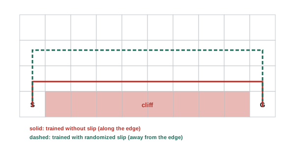
The policy trained in a perfect simulator learns the shortest path along the edge of the cliff. On a "real" robot that occasionally slips sideways, that path is deadly: about one run in five falls at 5 % slip, and two in three at 20 % slip. The policy trained with slip randomized between 0 and 30 % learns to take a longer route away from the edge; it is slightly slower, but its fall rate is far lower. This is domain randomization: training across a range of conditions wide enough that the real world looks like just another variation.

Closing the gap

Practitioners combine several techniques:

• Domain randomization of physical parameters (masses, friction, motor strength, delays), sensor noise and, for vision, lighting, textures and camera poses.
• System identification: measuring real parameters and making the simulator match them, including learned actuator models (actuator networks) trained on real motor data.
• Realistic latency and control rates in simulation, matching the real robot's computing pipeline.
• Observation choices that transfer well: proprioception transfers better than raw images, so many locomotion policies use only joint and IMU data, or height maps rather than pixels.
• Fine-tuning on real data, carefully and safely, after simulation training.
• Testing progressively: first in simulation with randomization, then with the robot suspended or in a safe test area, then in increasingly realistic conditions.

Privileged teacher-student training

Simulators know things real robots cannot sense: exact friction, terrain geometry under the feet, external forces, object masses. A powerful technique trains a teacher policy with access to this privileged information, which learns quickly and well, then trains a student policy that sees only realistic sensor data to imitate the teacher. The student learns to infer hidden properties from its history of observations, for example estimating ground slipperiness from how its feet have been moving. This approach, combined with large-scale randomization, has produced quadruped controllers that walk robustly over snow, mud, stairs and rubble, and humanoid controllers capable of agile and recovery behaviors.

Model-based reinforcement learning

Model-free RL needs huge amounts of experience. Model-based RL learns a dynamics model from data and uses it to plan or to generate imagined experience for policy training. World-model approaches (such as the Dreamer family) learn compact latent models from images and train policies inside them, achieving much better sample efficiency, which makes learning directly on real robots more feasible. Learned models can also be combined with MPC (Lesson 8). The risk is model bias: the policy can exploit errors in the learned model, just as it exploits simulator errors, so uncertainty-aware models and regular real-world data collection are used to keep models honest.

Safety in learning and deployment

Learned policies can behave unexpectedly in situations outside their training distribution, and exploration on real hardware can damage the robot or its surroundings. Safe practice includes training primarily in simulation; enforcing hard limits on joint positions, velocities and torques in low-level controllers that the policy cannot override; safety monitors that trigger a safe stop when states leave expected bounds; staged hardware testing with emergency stops and supervision; and logging of real-world behavior to find and fix failure cases. Policies for robots that work near people require additional safety measures and assessments (Lesson 12).