State estimation and sensor fusion

No sensor tells a robot exactly where it is or how fast it is moving. Wheel odometry drifts, IMUs drift faster, GPS jumps by meters and disappears indoors, and cameras lose track in featureless corridors. State estimation combines a model of how the robot moves with measurements from several imperfect sensors to produce the best estimate of the state, together with an honest measure of its uncertainty. That uncertainty matters as much as the estimate: a planner that knows its position is uncertain by half a meter can slow down near obstacles, and a manipulation system that knows an object pose is uncertain can choose a more forgiving grasp. This lesson introduces the probabilistic view of estimation, the Bayes filter, the Kalman filter and its nonlinear extensions, complementary filters for orientation, fusion of odometry, IMU and absolute sensors, outlier rejection, and smoothing with factor graphs.

The probabilistic view

Probabilistic robotics represents what the robot knows as a probability distribution over possible states, called the belief. The Bayes filter updates the belief in two steps that repeat forever:

• Prediction: apply the motion model to the previous belief, accounting for control inputs and process noise. Uncertainty grows, because motion is never perfectly known.
• Update (correction): incorporate a new measurement using the measurement model, weighting the prediction by how likely the measurement is for each possible state. Uncertainty shrinks.

Different filters represent the belief differently: Kalman filters use Gaussians (a mean and covariance), particle filters use sets of samples (Lesson 6), and grid filters use discretized histograms.

The Kalman filter

For linear models with Gaussian noise, the Kalman filter is the optimal Bayes filter. With state x, covariance P, motion model F, process noise Q, measurement model H and measurement noise R, each cycle computes:

The Kalman gain K balances trust between prediction and measurement: if measurements are noisy (large R), K is small and the filter relies on its model; if the prediction is uncertain (large P), K is large and the filter follows the measurement. The term z − Hx̂⁻ is the innovation, the surprise in the new measurement.

import numpy as np
# Kalman filter tracking a robot moving along a corridor from noisy position fixes
rng = np.random.default_rng(5)
dt, n = 0.1, 200
F = np.array([[1, dt], [0, 1]])          # constant-velocity motion model
H = np.array([[1.0, 0.0]])               # we measure position only
q = 0.05                                  # process noise (unmodeled acceleration)
Q = q * np.array([[dt ** 3 / 3, dt ** 2 / 2], [dt ** 2 / 2, dt]])
R = np.array([[0.5 ** 2]])                # measurement noise: 0.5 m standard deviation

true = np.zeros((n, 2)); true[0] = [0, 1.0]
for k in range(1, n):
    accel = 0.3 * np.sin(k * dt / 3)
    true[k] = F @ true[k - 1] + np.array([0.5 * dt ** 2, dt]) * accel
meas = true[:, 0] + rng.normal(0, 0.5, n)
dropout = range(100, 130)                 # no position fixes for 3 seconds

x = np.array([0.0, 0.0]); P = np.diag([1.0, 1.0])
est, sd = [], []
for k in range(n):
    x = F @ x; P = F @ P @ F.T + Q                       # predict
    if k not in dropout:
        y = meas[k] - H @ x                               # innovation
        S = H @ P @ H.T + R
        Kg = P @ H.T @ np.linalg.inv(S)                   # Kalman gain
        x = x + (Kg @ y).ravel(); P = (np.eye(2) - Kg @ H) @ P
    est.append(x.copy()); sd.append(np.sqrt(P[0, 0]))
est, sd = np.array(est), np.array(sd)
ok = [k for k in range(20, n) if k not in dropout]
print(f"raw measurement error (RMS): {np.sqrt(np.mean((meas[ok] - true[ok, 0]) ** 2)):.3f} m")
print(f"filtered position error (RMS): {np.sqrt(np.mean((est[ok, 0] - true[ok, 0]) ** 2)):.3f} m")
print(f"filtered velocity error (RMS): {np.sqrt(np.mean((est[ok, 1] - true[ok, 1]) ** 2)):.3f} m/s (velocity is never measured)")
print(f"position std before dropout {sd[99]:.2f} m, at end of dropout {sd[129]:.2f} m, 1 s after {sd[139]:.2f} m")

raw measurement error (RMS): 0.491 m
filtered position error (RMS): 0.306 m
filtered velocity error (RMS): 0.311 m/s (velocity is never measured)
position std before dropout 0.20 m, at end of dropout 1.09 m, 1 s after 0.20 m

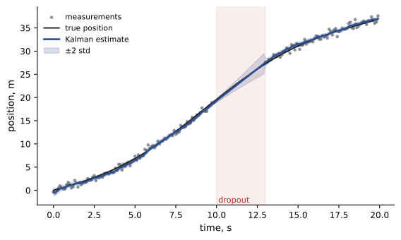
The filter reduces position error from about 0.49 m in the raw measurements to about 0.31 m, and it estimates velocity even though velocity is never measured, because the motion model links position changes to velocity. During the three-second dropout, the filter keeps predicting, and its position uncertainty grows from 0.2 m to over 1 m; when measurements return, uncertainty collapses again within a second. A well-tuned filter's reported uncertainty should match its actual errors. Here the filtered error is somewhat larger than the reported standard deviation, a sign that the process noise Q is set too low for the robot's real accelerations, so the filter is overconfident. Checking this consistency, for example with the normalized estimation error squared (NEES) in simulation, is an important tuning step.

Nonlinear filters

Real robots are nonlinear: a wheeled robot's position depends on the cosine and sine of its heading, and a range-bearing measurement to a landmark depends nonlinearly on the robot pose. Two common extensions handle this:

• The extended Kalman filter (EKF) linearizes the motion and measurement models around the current estimate using their Jacobians, then applies the Kalman equations. It is efficient and widely used, including in many drone and vehicle autopilots, but can diverge if the linearization is poor or the initial estimate is far off.
• The unscented Kalman filter (UKF) propagates a small set of carefully chosen sample points (sigma points) through the nonlinear functions and recovers the mean and covariance from them, often more accurate than the EKF for strongly nonlinear systems without needing Jacobians.

Error-state formulations, which estimate small errors around a nominal trajectory, are standard for IMU-based navigation because orientation is better handled as a small rotation error than as raw angles or quaternion components.

Orientation and the complementary filter

Estimating orientation from an IMU illustrates sensor fusion simply. Gyroscopes measure angular velocity accurately over short times, but integrating them drifts. Accelerometers measure gravity (when the robot is not accelerating) and give an absolute but noisy tilt reference. A complementary filter blends them: high-pass the gyro-integrated angle and low-pass the accelerometer angle, θ = α(θ + ω dt) + (1 − α) θ_acc, with α close to 1 (for example 0.98). The result follows quick motions from the gyro while slowly correcting drift with the accelerometer. Magnetometers correct heading drift but are disturbed by nearby steel and motors. More sophisticated orientation filters (Mahony, Madgwick, or EKF-based) follow the same idea.

Fusing odometry, IMU and absolute sensors

Mobile robots typically fuse several sources in an EKF or UKF:

• Wheel odometry: good short-term relative motion, but slips on smooth or loose surfaces and accumulates error in heading.
• IMU: high-rate angular velocity and acceleration, filling gaps between slower sensors and detecting slips.
• Visual or lidar odometry: estimates motion by tracking features or aligning scans between frames.
• Absolute measurements: GNSS outdoors (with RTK corrections for centimeter accuracy), localization against a map (Lesson 6), or fiducial markers and beacons indoors.

Relative sensors constrain how the robot moves; absolute sensors stop the drift. In ROS 2, the robot_localization package provides EKF and UKF nodes for this kind of fusion, typically producing a smooth odometry frame for control and a map-referenced frame for navigation.

Outliers and gating

Real sensors occasionally produce wildly wrong measurements: a GNSS multipath jump between buildings, a lidar return from a passing person, a misdetected landmark. Feeding such outliers into a Kalman filter drags the estimate away. Gating rejects measurements whose innovation is improbable under the filter's own uncertainty, using the Mahalanobis distance d² = yᵀ S⁻¹ y compared with a chi-square threshold (for example 9.21 for two-dimensional measurements at 99 %). Robust cost functions in optimization-based estimators serve a similar purpose. Gating requires an honestly calibrated uncertainty; an overconfident filter will reject good measurements and lose track.

Smoothing and factor graphs

Filters process each measurement once and keep only the current state. Smoothing methods instead keep a window or the full history of states and solve for the trajectory that best explains all measurements, typically as a nonlinear least-squares problem represented as a factor graph: nodes are states (poses, velocities, landmarks), and factors are measurements or motion constraints linking them. Libraries such as GTSAM, Ceres and g2o solve these problems efficiently by exploiting sparsity. Smoothing is more accurate than filtering because it can revise past estimates when new information arrives, which is essential for SLAM loop closures (Lesson 6) and for visual-inertial odometry, where sliding-window smoothers are standard.

Learning and estimation

Learning complements estimation rather than replacing it. Neural networks provide measurements (detected keypoints, learned depth, learned odometry) whose uncertainties can be estimated and fused; learned motion models capture effects such as wheel slip on different terrains; and some end-to-end policies estimate the state implicitly from sensor histories. Even then, explicit estimators remain valuable for their interpretability, uncertainty reporting and robustness, and most deployed robots use them for core localization.

Practical estimation work also involves checking sensor data quality before fusion: verifying timestamps, detecting stuck or saturated readings, and monitoring innovations over time. A sudden increase in innovation size often indicates a sensor fault, a miscalibration or a change in the environment, and logging these statistics helps diagnose problems in deployed robots.

A final practical point concerns coordinate frames in estimation. Fused estimates are usually published in two frames: a smooth, continuous odometry frame that never jumps, used for control, and a map frame that is corrected by absolute measurements and may jump slightly when corrections arrive. Keeping these separate prevents controllers from reacting violently to sudden localization corrections.

Estimation quality is ultimately judged by the tasks it supports: a localization error of 10 cm may be fine for a hallway delivery robot but unacceptable for docking with a charger or picking from a narrow shelf, so accuracy requirements should be set from the application.