Inverse kinematics, Jacobians and dynamics

Forward kinematics answers where the tool is for given joint angles. Most tasks pose the opposite question: the robot must place its gripper at a grasp pose computed by the perception system, so it needs the joint angles that achieve that pose. This is inverse kinematics (IK), and it is harder than forward kinematics: there may be several solutions, infinitely many, or none at all. Closely related is the Jacobian, which relates joint velocities to tool velocities and is the foundation of velocity control, singularity analysis and force control. Beyond geometry, real robots have mass and inertia, so moving them requires torques that depend on their dynamics. This lesson covers analytic and numerical inverse kinematics, the Jacobian and its uses, singularities and manipulability, redundancy resolution, and an introduction to manipulator dynamics and its role in control and simulation.

The inverse kinematics problem

Given a desired tool pose, inverse kinematics finds joint values q such that FK(q) equals the desired pose. Several situations arise:

• Multiple solutions: a planar two-link arm can reach most points with elbow up or elbow down; a typical six-joint industrial arm can have up to eight (and in general up to sixteen) solutions for a given pose, corresponding to shoulder, elbow and wrist configurations.
• Infinite solutions: redundant arms (seven or more joints for a 6D task) have a continuous family of solutions, called the self-motion manifold.
• No solution: the pose is outside the workspace, or violates joint limits.

The IK solver must also choose among solutions sensibly: staying close to the current configuration, respecting joint limits, avoiding collisions and singularities.

Analytic and numerical solutions

For many arm geometries, closed-form analytic solutions exist. For the planar two-link arm, the law of cosines gives the elbow angle, and the shoulder angle follows from geometry. Industrial arms with spherical wrists (three wrist axes intersecting at a point) have analytic solutions that separate wrist position from orientation, and solver generators such as IKFast derive them automatically. Analytic solutions are fast and return all solutions.

Numerical methods work for any robot. Starting from an initial guess, they repeatedly compute the tool pose error and update the joints using the Jacobian. The Jacobian inverse or pseudo-inverse update Δq = J⁺ e can become unstable near singularities, so practical solvers use damped least squares (also called Levenberg-Marquardt):

where e is the pose error and λ is a damping factor that trades accuracy for stability near singularities. Optimization-based IK solvers (for example TRAC-IK or solvers in Drake and MoveIt) add joint limits, collision avoidance and secondary objectives as constraints or costs.

import numpy as np
# Inverse kinematics of a planar two-link arm: analytic solution and Jacobian iteration
l1, l2 = 0.5, 0.4

def fk(q):
    return np.array([l1 * np.cos(q[0]) + l2 * np.cos(q[0] + q[1]),
                     l1 * np.sin(q[0]) + l2 * np.sin(q[0] + q[1])])

def jacobian(q):
    s1, c1 = np.sin(q[0]), np.cos(q[0])
    s12, c12 = np.sin(q[0] + q[1]), np.cos(q[0] + q[1])
    return np.array([[-l1 * s1 - l2 * s12, -l2 * s12],
                     [l1 * c1 + l2 * c12, l2 * c12]])

def analytic(x, y, elbow=1):
    c2 = (x * x + y * y - l1 * l1 - l2 * l2) / (2 * l1 * l2)
    q2 = elbow * np.arccos(np.clip(c2, -1, 1))
    q1 = np.arctan2(y, x) - np.arctan2(l2 * np.sin(q2), l1 + l2 * np.cos(q2))
    return np.array([q1, q2])

def dls(target, q0, lam=0.05, iters=100):
    q = np.array(q0, dtype=float)
    for i in range(iters):
        err = target - fk(q)
        if np.linalg.norm(err) < 1e-5:
            return q, i
        J = jacobian(q)
        q += J.T @ np.linalg.solve(J @ J.T + lam ** 2 * np.eye(2), err)   # damped least squares
    return q, iters

target = np.array([0.6, 0.3])
for elbow in (1, -1):
    q = analytic(*target, elbow)
    print(f"analytic elbow {elbow:+d}: q = {np.degrees(q).round(1)} deg, reaches {fk(q).round(4)}")
q, n = dls(target, [0.1, 0.1])
print(f"damped least squares from (0.1, 0.1): q = {np.degrees(q).round(1)} deg after {n} iterations")

for q2 in (np.radians(90), np.radians(10), np.radians(1)):
    J = jacobian([0.3, q2])
    print(f"q2 = {np.degrees(q2):5.1f} deg: det(J) = {np.linalg.det(J):.4f}, smallest singular value {np.linalg.svd(J)[1].min():.4f}")

analytic elbow +1: q = [-9.8 84.3] deg, reaches [0.6 0.3]
analytic elbow -1: q = [ 63.  -84.3] deg, reaches [0.6 0.3]
damped least squares from (0.1, 0.1): q = [-9.8 84.3] deg after 5 iterations
q2 =  90.0 deg: det(J) = 0.2000, smallest singular value 0.2863
q2 =  10.0 deg: det(J) = 0.0347, smallest singular value 0.0354
q2 =   1.0 deg: det(J) = 0.0035, smallest singular value 0.0035

The analytic solver returns both elbow configurations for the target (0.6, 0.3) m. The numerical solver, started from a nearly straight arm, converges in five iterations to the elbow-up solution, the one nearest its starting guess; a different initial guess could produce the other solution. The last lines show what happens as the elbow straightens: the Jacobian's determinant and smallest singular value approach zero, which is the signature of a singularity.

The Jacobian

The Jacobian J(q) is the matrix of partial derivatives of the tool pose with respect to the joints. It maps joint velocities to tool velocities:

For a six-DOF arm, J is 6 × 6, with rows for linear and angular velocity. The Jacobian has several uses:

• Velocity control: commanding the tool to move at a desired velocity by solving for joint velocities, as in teleoperation and visual servoing.
• Numerical IK, as above.
• Force mapping: by the principle of virtual work, joint torques τ that produce a tool force F are τ = Jᵀ F, used in force control and in estimating contact forces from joint torque sensors.
• Singularity and dexterity analysis.

Singularities and manipulability

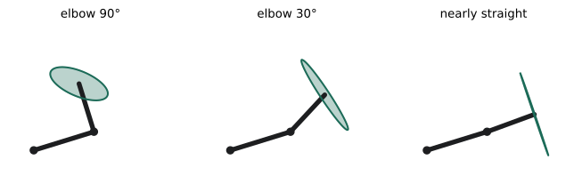
A singularity is a configuration where the Jacobian loses rank: the tool cannot move in some direction no matter how the joints move, and near the singularity, small tool motions require very large joint velocities. Common singularities include a fully stretched arm (boundary singularity), wrist singularities when two wrist axes align, and shoulder singularities when the wrist center lies on the first joint axis. Near singularities, velocity commands can produce dangerous joint speeds, so controllers detect them and slow down, damp the solution, or plan paths that avoid them.

Manipulability, w = √det(J Jᵀ), measures how far a configuration is from singularity; it is zero at singularities and larger in dexterous configurations. Visualized as an ellipsoid, it shows in which directions the tool can move easily. Planners can favor high-manipulability postures for tasks requiring fine motion in all directions.

Redundancy resolution

A redundant arm can satisfy the main task while using its extra freedom for secondary goals. With the Jacobian pseudo-inverse, the general solution is q̇ = J⁺ ẋ + (I − J⁺ J) z, where the second term moves the joints in the null space of the Jacobian, changing the arm's posture without moving the tool. The vector z can be chosen to move away from joint limits, avoid obstacles with the elbow, or increase manipulability. Task-priority and whole-body control frameworks extend this idea to humanoids and mobile manipulators with many simultaneous tasks: keep balance first, then keep the hand on target, then keep the head looking at the object, and so on.

Dynamics

Kinematics ignores forces. To move an arm, the motors must supply torques that accelerate the links, overcome gravity, and handle velocity-dependent effects. The manipulator equation of motion is:

where M is the configuration-dependent mass (inertia) matrix, C contains Coriolis and centrifugal terms, g is the gravity torque vector, τ are the joint torques and F_ext are external forces at the tool. Efficient algorithms (such as the recursive Newton-Euler algorithm for inverse dynamics and the articulated body algorithm for forward dynamics) compute these terms in time proportional to the number of joints, enabling real-time control and fast simulation.

Dynamics models are used for gravity compensation (holding an arm still with exactly the torque needed), computed-torque and feedforward control that cancel known dynamics so feedback only corrects errors, collision detection by comparing expected and measured torques, and simulation. Models require accurate masses, centers of mass and inertias, which are estimated by system identification experiments.

Kinematics and learning

Learning-based robot controllers often still rely on kinematics. Many learned manipulation policies output desired end-effector poses or velocities, which an IK or operational-space controller converts into joint commands; others output joint positions directly. Learned IK networks can provide fast initial guesses for numerical solvers, and differentiable kinematics and dynamics allow gradients to flow through robot models during training. Understanding the underlying geometry helps diagnose learned policies that command impossible or singular poses.

Inverse kinematics in practice

In real systems, IK is called many times per second, for example to convert each waypoint of a planned Cartesian path into joint targets or to servo the gripper toward a moving object. Several practical issues arise. Consecutive solutions must be consistent, because jumping between elbow-up and elbow-down configurations mid-motion would swing the arm violently; solvers therefore start from the current configuration and penalize large joint changes. Joint limits, including limits on continuous rotation of wrist joints, must be respected. Orientation and position errors have different units, so they must be weighted sensibly in the error vector. And when a target is unreachable, the solver should return the closest feasible pose and report failure rather than silently producing a poor result.

For mobile manipulators, the base and arm together form a redundant system. Whole-body IK can choose whether to reach by moving the arm, the base or both, trading off speed, stability and accuracy, which is a common source of natural-looking motion in modern service robots.

Finally, remember that kinematic and dynamic models are approximations. Flexible links, gear compliance, cable forces and temperature changes all cause the real robot to deviate from its model. High-precision applications such as machining or surgery compensate with calibration, external measurement (for example laser trackers or cameras) and closed-loop correction at the tool.