Cost and infrastructure

Machine learning can be expensive. Accelerators cost thousands of dollars a month each, training runs can consume thousands of GPU hours, and an inefficient online service can cost more to run than the value it creates. At the same time, infrastructure decisions, such as cloud or on-premises, CPUs or GPUs, shared clusters or dedicated machines, determine how quickly teams can experiment. This lesson covers the infrastructure that ML systems run on, the main cost drivers in training and serving, how to estimate cost per prediction, purchasing options such as spot and reserved capacity, and the practices, often called FinOps, that keep spending visible and under control. All prices in this lesson are illustrative; real prices vary by provider, region and time.

The infrastructure stack

Most organizations run ML on a layered stack:

• Compute: CPU servers for data processing, classical models and serving; GPUs or other accelerators (such as TPUs or custom inference chips) for deep learning training and serving.
• Storage: object storage for datasets and artifacts, data warehouses and lakes, and fast local or network storage for training data feeds.
• Orchestration: Kubernetes has become the common substrate for running containers, with ML-specific layers (Kubeflow, Ray, KServe) and batch schedulers (Slurm in research clusters) on top.
• Platforms: managed ML services from cloud providers that bundle notebooks, training jobs, registries, endpoints and monitoring; and internal platforms built by MLOps teams from open-source components.

Organizations choose between public cloud (elastic, quick to start, broad services, pay as you go), on-premises or colocated hardware (lower unit cost at high, steady utilization, data control, but capital investment and slower change), and hybrids. For many, the deciding factors are utilization and data gravity: large, steady GPU workloads may be cheaper on owned hardware, while variable or experimental workloads benefit from the cloud's elasticity, and moving petabytes of data between locations is itself costly.

What drives cost

Training costs scale with the amount of computation and the price of the hardware, plus storage and data movement, plus the cost of failed or abandoned experiments, which often exceeds the cost of the final training run. Serving costs scale with traffic, the compute per prediction, and, crucially, utilization: a GPU that is idle 70 % of the time costs the same as one that is busy. Hidden costs include data pipelines and feature stores running continuously, logging and monitoring storage, network egress between regions or clouds, and engineers' time.

Cost per prediction

The most useful serving metric for cost decisions is the cost per prediction (or per thousand or million predictions): the hourly cost of a replica divided by the predictions it actually serves per hour, which depends on its throughput at the latency SLO and on its average utilization.

# Illustrative costs (not quotes): cost per million predictions for three serving options
options = {
    # name: (hourly price, requests per second at the SLO, average utilization achieved)
    "CPU, 8 vCPU, tree model":     (0.40,  900, 0.55),
    "GPU, small, batched CNN":     (1.20, 1400, 0.45),
    "GPU, large, unbatched CNN":   (4.00,  300, 0.45),
}
print("Option                        cost per million predictions")
for name, (price, rps, util) in options.items():
    per_hour = rps * 3600 * util
    print(f"{name:<30}{price / per_hour * 1e6:10.2f}")

# Training a model on spot capacity with interruptions and checkpoints
gpu_hours, on_demand, spot = 2000, 3.00, 1.10
interruptions_per_100h, lost_h_each = 6, 0.5          # work lost back to the last checkpoint
spot_hours = gpu_hours * (1 + interruptions_per_100h / 100 * lost_h_each)
print(f"Training on demand: {gpu_hours * on_demand:,.0f}; on spot with interruptions: {spot_hours * spot:,.0f}")

# Reserved capacity versus on demand for a steady serving load
on_demand_hourly, reserved_hourly, hours = 1.00, 0.62, 8760
for used in (0.3, 0.6, 0.9):
    print(f"Fleet busy {used:.0%} of the year: on demand {used * hours * on_demand_hourly:,.0f} vs reserved {hours * reserved_hourly:,.0f} per instance")
print(f"Break-even utilization: {reserved_hourly / on_demand_hourly:.0%}")

Option                        cost per million predictions
CPU, 8 vCPU, tree model             0.22
GPU, small, batched CNN             0.53
GPU, large, unbatched CNN           8.23
Training on demand: 6,000; on spot with interruptions: 2,266
Fleet busy 30% of the year: on demand 2,628 vs reserved 5,431 per instance
Fleet busy 60% of the year: on demand 5,256 vs reserved 5,431 per instance
Fleet busy 90% of the year: on demand 7,884 vs reserved 5,431 per instance
Break-even utilization: 62%

The tree model on a CPU costs about 0.22 per million predictions. A batched image model on a small GPU costs about 0.53, while the same kind of model on a large GPU without batching costs over 8, almost 40 times the CPU option, because it serves few requests per hour for a high price. The lesson is that the hardware price alone tells little; throughput at the SLO and utilization dominate. Batching, right-sizing (using the smallest hardware that meets the SLO), and autoscaling to keep utilization up (Lesson 6) are usually the largest savings available.

Purchasing options

Cloud providers sell capacity in several ways. On-demand instances can be started and stopped at any time at the highest hourly price. Reserved instances or committed-use discounts give a lower price in exchange for a one- or three-year commitment, and pay off only if the capacity is used enough: in the illustration, reserving at 62 % of the on-demand price breaks even at 62 % utilization over the year, so it suits steady base load, not peaks. Spot (or preemptible) instances use spare capacity at deep discounts but can be reclaimed with little warning. They suit fault-tolerant work such as training with frequent checkpoints, batch scoring and hyperparameter searches: in the illustration, a 2,000 GPU-hour training job costs 6,000 on demand and about 2,300 on spot, even after redoing work lost at interruptions. A typical portfolio covers steady serving with reserved capacity, peaks with on-demand, and training and batch jobs with spot.

Shared clusters and scheduling

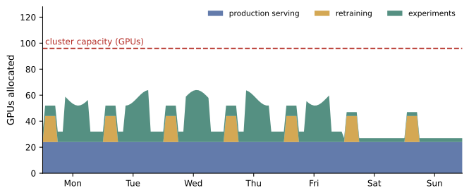
Accelerators are expensive, so organizations pool them in shared clusters rather than giving each team dedicated machines that sit idle at night. A scheduler allocates GPUs to jobs according to priorities and quotas: production serving and retraining first, then team experiments, with fair sharing among teams. Techniques such as job queueing, preemption of low-priority jobs, packing several small jobs on one GPU (with features such as NVIDIA Multi-Instance GPU), and automatically shutting down idle notebooks raise utilization. Measuring utilization per team and per job is the first step: many organizations discover that their expensive GPUs are busy less than half the time.

FinOps for ML

FinOps is the practice of making cloud costs visible and accountable. For ML, it means tagging every resource with its team, project and model; reporting cost per model and per prediction alongside accuracy; setting budgets and alerts on training projects; reviewing large training runs before they start; and making cost a factor in model selection (Lesson 3). A model that is 0.2 % more accurate but costs five times as much to serve is rarely the right choice, and that trade-off should be explicit. Engineers who can see the cost of their experiments typically find large savings quickly.

Energy and carbon

ML workloads consume significant electricity, and organizations increasingly report and reduce their emissions. The emissions of a workload depend on the energy it uses (hardware power multiplied by time, plus data center overhead, measured by PUE) and on the carbon intensity of the electricity, which varies enormously by region and time of day: a GPU-hour in a region powered mainly by hydroelectricity or nuclear emits a small fraction of one powered by coal. Running flexible training jobs in low-carbon regions or hours, improving utilization, and choosing efficient models and hardware all cut emissions as well as cost.

In the United States, grid carbon intensity varies widely by region: the Pacific Northwest (hydroelectric) and areas with large nuclear or renewable shares are low, while regions relying on coal are high. Location choices for compute therefore matter, and climate disclosure rules, notably California's laws for large companies, are developing.

Estimating training cost

Before a large training run, it is worth estimating its cost. For neural networks, a common approximation is that training a model with N parameters on D tokens or examples needs about 6ND floating-point operations; dividing by the hardware's achieved throughput (a realistic fraction, often 30 to 50 %, of its peak) gives the accelerator time. For example, a 1-billion-parameter model trained on 20 billion tokens needs about 1.2 × 10²⁰ operations; at an achieved 300 teraflops per accelerator, that is about 400,000 accelerator-seconds, or roughly 110 accelerator-hours. For classical models, a timed run on a sample, scaled up, gives a quick estimate. Adding the expected number of experiments, failed runs and hyperparameter searches, often several times the cost of the final run, gives a budget that can be compared with the expected value of the model.

Storage and data movement deserve a line in every estimate. Keeping many versions of large datasets and checkpoints in fast storage is costly, so lifecycle policies move older artifacts to cheaper archive tiers and delete what is no longer needed, while retaining what reproducibility and audit require.

Cost reviews are most useful when they are routine. A monthly review of the largest cost items per model, with the owners present, usually finds idle endpoints, oversized instances, forgotten experiments and storage that can be archived, and it keeps cost in view when new models are designed.