Monitoring, drift and retraining

Deploying a model is the start of its working life, and that life is spent in a world that keeps changing. Customers change their habits, competitors change prices, fraudsters change tactics, upstream systems change formats, and a pandemic or a recession can change everything at once. A model that was accurate at release can degrade quietly, and because ML failures are silent (Lesson 1), nobody notices unless the system is watched. This lesson covers what to monitor, the different kinds of drift, how to detect them statistically, what to do when labels arrive late, how to design alerts that people act on, and when and how to retrain.

What to monitor

Monitoring an ML system covers four layers, from the most immediate to the most meaningful:

• Service health: request rate, error rate, latency percentiles, resource use, the standard signals of any online service (Lesson 6).
• Data: the distribution of each input feature, missing value rates, out-of-range values and schema violations, compared with the training data or a recent reference window.
• Predictions: the distribution of model outputs, such as the share of transactions flagged as fraud or the mean predicted price. A sudden change in output distribution is often the first sign of trouble, as in the cents-versus-dollars bug of Lesson 1.
• Outcomes: model quality measured against actual labels when they arrive, and the business metrics the model is meant to improve.

Service health and data monitoring are available immediately; outcome monitoring may wait days or months for labels. A complete monitoring design uses all four.

Kinds of drift

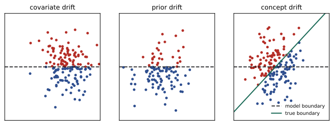
A model learns the relationship between inputs X and target y from training data. Drift is any change in the joint distribution P(X, y) after training. It helps to distinguish its forms:

• Covariate (data) drift: the distribution of inputs P(X) changes, but the relationship P(y | X) stays the same. A lender starts attracting younger applicants; the model may still be correct for each applicant but is now applied mostly in a region of the input space where it had little training data.
• Prior (label) drift: the base rate P(y) changes, for example the share of fraudulent transactions doubles during a holiday attack. Thresholds and calibrated probabilities may need adjustment.
• Concept drift: the relationship P(y | X) itself changes, so the same inputs now mean something different. Fraudsters learn which patterns are flagged and change behavior; a feature that predicted churn stops doing so after a product change. Concept drift is the most damaging and cannot be detected from inputs alone.

Drift can be sudden (a new regulation, a system change), gradual (slowly changing tastes), seasonal (recurring patterns the model should already know) or a one-off event. Data pipeline bugs, which are not real-world drift at all, look like sudden covariate drift and are among the most common causes of alerts.

Detecting drift

Distribution drift in a feature or prediction is detected by comparing a current window (say the last day) with a reference (the training data or a stable recent period). Common measures are:

• The population stability index (PSI), widely used in credit risk: bin the reference into, for example, deciles, and compare the share of current data in each bin.

where e and a are the expected (reference) and actual (current) shares in bin i. A common rule of thumb reads PSI below 0.1 as stable, 0.1 to 0.25 as a moderate shift worth investigating, and above 0.25 as a significant shift.

• The Kolmogorov-Smirnov (KS) statistic: the largest difference between the two cumulative distributions, with a test of whether they differ.
• For categorical features, the chi-squared test or the Jensen-Shannon divergence between category frequencies.

import numpy as np
from scipy.stats import ks_2samp

def psi(expected, actual, bins=10):
    # population stability index using decile bins of the reference data
    edges = np.quantile(expected, np.linspace(0, 1, bins + 1))
    edges[0], edges[-1] = -np.inf, np.inf
    e = np.histogram(expected, edges)[0] / len(expected)
    a = np.histogram(actual, edges)[0] / len(actual)
    e, a = np.clip(e, 1e-6, None), np.clip(a, 1e-6, None)
    return np.sum((a - e) * np.log(a / e))

rng = np.random.default_rng(5)
reference = rng.normal(50, 10, 50000)           # feature at training time
cases = {"same distribution": rng.normal(50, 10, 5000),
         "mean shift +2": rng.normal(52, 10, 5000),
         "mean shift +5": rng.normal(55, 10, 5000),
         "wider spread": rng.normal(50, 15, 5000)}
print("Case                 PSI     KS stat  KS p-value")
for name, x in cases.items():
    ks = ks_2samp(reference, x)
    print(f"{name:<20} {psi(reference, x):6.3f}  {ks.statistic:7.3f}  {ks.pvalue:9.2e}")

# A KS test on a huge sample flags trivial differences
big = rng.normal(50.3, 10, 500000)
print(f"Tiny shift +0.3 with 500,000 rows: PSI {psi(reference, big):.4f}, KS p-value {ks_2samp(reference, big).pvalue:.1e}")

Case                 PSI     KS stat  KS p-value
same distribution     0.001    0.012   5.34e-01
mean shift +2         0.036    0.079   3.82e-25
mean shift +5         0.225    0.193  3.61e-149
wider spread          0.198    0.107   5.26e-46
Tiny shift +0.3 with 500,000 rows: PSI 0.0007, KS p-value 1.7e-05

With no drift, PSI is essentially zero and the KS test finds nothing. A mean shift of 0.2 standard deviations gives PSI 0.04, below the investigation threshold, while a shift of half a standard deviation (PSI 0.23) and a 50 % wider spread (PSI 0.20) fall in the moderate band. The KS p-values, however, are tiny in all three drifted cases, and the last line shows the problem with significance tests on large samples: a shift of 0.03 standard deviations, which matters to no one, is "highly significant" with half a million rows. For monitoring, effect sizes such as PSI or the KS statistic itself are more useful than p-values, with thresholds tuned to the feature's importance and history.

Monitoring every feature with fixed thresholds generates noise. Practical systems prioritize: they watch the most important features (by feature importance), the prediction distribution, and data-quality signals closely, and review the rest in periodic reports.

When labels arrive late

Many targets are known only later: whether a loan defaults (months), whether a customer churns (weeks), whether a transaction was fraudulent (up to 90 days for chargebacks). During the delay, the model's accuracy is unknown. Teams use several strategies:

• Proxy metrics available sooner, such as early repayment behavior, manual review outcomes or user engagement.
• Prediction and input drift as early warnings, accepting that they cannot detect pure concept drift.
• Partial labels: measuring quality on the subset of cases whose labels have arrived, being careful that this subset may be biased (early chargebacks may differ from late ones).
• A small randomized holdout or human-labeled sample of recent traffic, which gives unbiased quality estimates at a cost.

Alerts that people act on

Monitoring is useful only if someone responds. The principles of alarm management from operations engineering apply: every alert should require a specific action, have an owner, and be rare enough to be taken seriously. Alerts are tiered: immediate pages for service failures and sudden large shifts in predictions (which often indicate a bug), and tickets or daily reports for gradual drift. Each alert should link to a runbook explaining how to investigate: check upstream data validation, compare against recent deployments, look at the affected feature's pipeline, and decide whether to roll back the model, fix the data, or retrain. Dashboards show trends for people investigating, but they do not replace alerts, because nobody watches dashboards at 3 a.m.

Retraining

Most production models are retrained regularly, because some drift is inevitable. Strategies include:

• Scheduled retraining (daily, weekly, monthly) on a sliding window of recent data, chosen by measuring how fast performance decays in backtests.
• Triggered retraining when monitoring detects drift or performance drops below a threshold.
• Online or incremental learning, updating the model continuously as new labeled data arrive, used for fast-changing problems such as ad click prediction, with careful safeguards against learning from corrupted data.

Retraining is not free and not automatically safe. A retrained model must pass the same tests and release gates as any new model (Lesson 4), because it can absorb a data bug or a temporary anomaly. Retraining also does not fix every problem: if a feature has become meaningless, or a feedback loop is shaping the labels, retraining on new data can make things worse. And a model retrained on data shaped by its own decisions (for example, loans approved only by the previous model) sees outcomes only for the cases it chose, a selection bias that may require randomized exploration or careful reweighting to correct.

Monitoring infrastructure

Monitoring needs data. Serving systems log every request with its timestamp, model version, input features (or a sample of them), prediction and latency, and later join the logged predictions to their eventual labels. These prediction logs are the raw material for drift detection, quality measurement, debugging and future training data, so they should be stored durably with appropriate privacy protection. Metrics are aggregated by tools such as Prometheus and visualized in dashboards such as Grafana, while specialized ML monitoring tools, open-source or commercial, compute drift statistics and slice-level quality. Sampling keeps costs manageable for high-volume services, but samples must be large enough to detect the shifts that matter on the slices that matter.

A final practical point concerns baselines for comparison. Comparing today's data with the original training set flags every seasonal change; comparing with the same day last week or last year, or with a rolling recent window, separates expected patterns from genuine surprises. Many teams monitor against both: the training reference for long-term drift that may justify retraining, and a recent window for sudden changes that may indicate a bug.