Experiment tracking, reproducibility and model registries

Developing a model means running many experiments: different features, algorithms, hyperparameters and data slices. Without discipline, the results end up scattered across notebooks, file names like model_final_v3_really_final.pkl, and the memories of whoever ran them. Six months later, no one can say which data and settings produced the model in production, or reproduce it to fix a bug. This lesson covers how to track experiments, what reproducibility requires, how to compare models fairly when results are noisy, and how a model registry manages the trained models that move toward production.

What to record for every run

An experiment tracking system records, for each training run, everything needed to understand and reproduce it:

• Code version: the Git commit of the training code, and a flag if there were uncommitted changes.
• Data version: identifiers or content hashes of the training, validation and test datasets (Lesson 2).
• Configuration: hyperparameters, feature list, preprocessing options and random seeds.
• Environment: library versions, container image, hardware type.
• Metrics: training and validation metrics, ideally over time (learning curves), and metrics on important data slices.
• Artifacts: the trained model file, plots, evaluation reports and sample predictions.
• Context: who ran it, when, why (a short note), and links to related runs.

Tools such as MLflow, Weights & Biases, Neptune and the tracking features of cloud ML platforms make this almost automatic: a few lines of code log parameters, metrics and artifacts to a central server with a searchable interface. The habit matters more than the tool. A run that is not logged did not happen.

Reproducibility

A result is reproducible if someone else, or you later, can rerun the same code on the same data in the same environment and get the same result. In ML, several things work against this:

• Randomness in data splits, initialization, dropout, data shuffling and sampling, controlled by fixing and logging random seeds.
• Non-deterministic computation on GPUs, where some parallel operations add numbers in varying order; frameworks offer deterministic modes at some cost in speed.
• Changing data, solved by versioned, immutable datasets.
• Changing environments: a new library version can change default parameters or numerical results, solved by pinned dependency versions and container images.
• Hidden state: notebooks run out of order, global variables, and files read from personal directories. Production training should run as scripts or pipelines from a clean environment.

Perfect bit-for-bit reproducibility is not always achievable or necessary, especially on GPUs, but the result should be reproducible to within the run-to-run noise, and that noise must be known.

Comparing models when results are noisy

Every evaluation score is a random quantity: it depends on the random split of the data, the random seed of training, and the particular test examples. Comparing two models on a single run can easily pick the wrong one.

import hashlib, json
import numpy as np
from sklearn.datasets import make_classification
from sklearn.model_selection import train_test_split
from sklearn.ensemble import RandomForestClassifier

X, y = make_classification(n_samples=3000, n_features=20, n_informative=6, flip_y=0.08, random_state=7)
data_hash = hashlib.sha256(X.tobytes() + y.tobytes()).hexdigest()[:12]

def run(depth, seed):
    Xtr, Xte, ytr, yte = train_test_split(X, y, test_size=0.3, random_state=seed)
    m = RandomForestClassifier(n_estimators=100, max_depth=depth, random_state=seed)
    return m.fit(Xtr, ytr).score(Xte, yte)

results = {}
for depth in (7, 8):
    config = {"model": "random_forest", "max_depth": depth, "n_estimators": 100, "data": data_hash}
    run_id = hashlib.sha256(json.dumps(config, sort_keys=True).encode()).hexdigest()[:8]
    results[depth] = np.array([run(depth, s) for s in range(10)])
    r = results[depth]
    print(f"depth {depth}: config {run_id}, data {data_hash}; seed 0 = {r[0]:.3f}; "
          f"10 seeds = {r.mean():.3f} +/- {r.std(ddof=1):.3f}")

diff = results[8] - results[7]
print(f"Paired difference (depth 8 minus 7): mean {diff.mean():+.4f}, positive in {(diff > 0).sum()} of 10 seeds")

depth 7: config d09a6937, data 4d8810776f53; seed 0 = 0.851; 10 seeds = 0.834 +/- 0.010
depth 8: config 1fe883fc, data 4d8810776f53; seed 0 = 0.844; 10 seeds = 0.841 +/- 0.011
Paired difference (depth 8 minus 7): mean +0.0070, positive in 7 of 10 seeds

On seed 0, the depth-7 forest scores 0.851 and the depth-8 forest 0.844, so a single run would favor depth 7. Across ten seeds, depth 8 is better on average (0.841 against 0.834) and wins on 7 of the 10 paired comparisons. The standard deviation across seeds, about 0.01, is larger than the difference between the models. The lessons are to evaluate candidates on several seeds or cross-validation folds, to compare them on the same splits (a paired comparison, which cancels much of the split-to-split noise), and to report variation as well as means. When the difference is smaller than the noise, other considerations, such as speed, simplicity or interpretability, should decide.

The output also shows two short hashes. The configuration hash identifies the exact settings, and the data hash identifies the exact dataset; logging both with the scores means anyone can tell whether two runs are truly comparable.

Hyperparameter search

Choosing hyperparameters is itself an experiment, often with hundreds of runs. Grid search tries every combination of a few values, which wastes runs on unimportant parameters. Random search samples combinations at random and usually finds good settings faster, because only a few hyperparameters typically matter. Bayesian optimization (for example with Optuna or Hyperopt) builds a model of how the score depends on the hyperparameters and proposes promising settings, and early-stopping methods such as successive halving and Hyperband abandon poor runs quickly to save compute. Whatever the method, the search must use a validation set, never the final test set, or the reported test score will be optimistic: with enough tries, some configuration will do well on the test set by chance.

The model registry

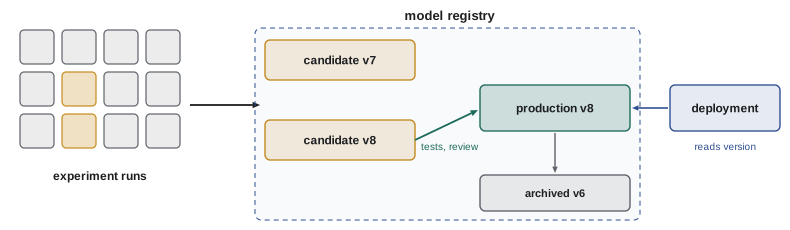
Once a model is worth considering for production, it moves from the experiment tracker into a model registry: a catalog of trained models with their versions, lineage (the run, code and data that produced them), evaluation results, documentation and status. Typical statuses are candidate (or staging), production, and archived, and transitions between them follow a defined process: a candidate becomes production only after passing tests (Lesson 4), review and, often, an online experiment (Lesson 8). Deployment systems read the registry to find which version to serve, so promoting or rolling back a model is a registry change rather than a manual file copy (Lesson 5).

Each registered model should come with a model card: a short document stating what the model does, its intended uses and limits, the data it was trained on, its performance overall and on relevant subgroups, and known risks. Model cards, introduced by Mitchell and colleagues in 2019, are now a common expectation in governance frameworks (Lesson 11).

Notebooks and production code

Notebooks are excellent for exploration but poor as production artifacts: hidden state, out-of-order execution, difficulty of testing and code review. A common practice is to explore in notebooks, then move stable code (feature transformations, training loops, evaluation) into version-controlled Python modules with tests, which both the notebooks and the production pipelines import. Training in production then runs as a script or pipeline step with all inputs specified explicitly, its outputs logged to the tracker and registered models produced automatically (Lesson 10).

Lineage and audit

For any prediction a production model makes, an organization should be able to answer: which model version made it, what code and data trained that version, who approved its release, and what evaluation it passed. This lineage chain, from prediction through serving logs, registry, tracker and data versions, is essential for debugging, for responding to complaints and for regulatory audits. It is built from the habits in this lesson: log every run, version every dataset, register every candidate, and record every promotion.

Environments and dependency pinning

Many reproducibility failures come from the software environment rather than the code. A training script that ran last year may now fail, or silently produce different results, because a library changed a default value, deprecated a function or altered a numerical routine. The defenses are well established. Pin exact versions of every dependency in a lock file (produced by tools such as pip-tools, Poetry or conda-lock), build training and serving images from those lock files, and record the image identifier with each run. Upgrade dependencies deliberately, as a change that goes through testing and a comparison run, rather than accidentally whenever someone rebuilds an environment. For GPU work, the driver, CUDA and framework versions belong in the record too, because they affect both speed and numerical results.

It is also worth recording the hardware. The same code can produce slightly different results on different GPU models, and very different training times; knowing that a run used eight accelerators of a particular type explains both its cost and its behavior.

Organizing experiments

Tracking tools become cluttered quickly, so teams adopt conventions. Runs are grouped into named experiments, each tied to a question ("does adding the support-ticket features help?"), with a short written hypothesis before the runs start and a conclusion afterwards. Tags mark runs that were exploratory, that used a debug subset, or that are candidates for registration. Dashboards compare runs within an experiment on the same metrics and slices. Periodic clean-up archives failed and abandoned runs while keeping their records. These habits turn the tracker from a log of everything into a searchable history of what the team learned, which is invaluable when new members join or when a decision made a year ago needs to be revisited.

Another useful habit is to keep a baseline run in every experiment: the current production configuration retrained on the same data. Comparing candidates with a fresh baseline, rather than with an old number recorded months earlier, ensures that any improvement comes from the change being tested and not from newer data or a changed evaluation set.