Governing equations of fluid flow

Prairiewind Aerospace has decided to give the Tern a new wing. The airline customers like the aircraft, but they want it to use shorter and rougher strips in western Kansas and Colorado, to burn less energy in cruise and to stall more gently when a pilot gets slow on a gusty approach. The first version of the wing was designed quickly, using handbook data and a lot of experience. The Block 2 wing will be designed properly, from the airfoil sections up. Tomasz Wierzbicki, who leads the aerodynamics group, has asked Arjun Mehta, now on his third co-op work term, to follow the design from start to finish. Arjun has met lift and drag coefficients in earlier courses. This course shows where those coefficients come from. It starts with the equations that every aerodynamic method, from a hand calculation to a supercomputer simulation, is built on.

Describing a flowing fluid

Air is made of molecules, but at the scale of a wing we never track them one by one. Instead we treat air as a continuum: a smooth substance whose density \(\rho\), pressure \(p\), temperature \(T\) and velocity \(\mathbf{V} = (u, v, w)\) have definite values at every point and every instant. The continuum idea works when the mean free path of the molecules, about 70 nanometers at sea level, is tiny compared with the smallest length that matters, such as the thickness of a boundary layer. It fails only in very thin gas, high in the atmosphere or in some microdevices, which is not the Tern's world.

There are two ways to describe the motion. In the Lagrangian view, we follow individual fluid particles and record what happens to each one. In the Eulerian view, we stand at fixed points and record the velocity, pressure and density of whatever fluid is passing. Wind tunnels and computer programs almost always use the Eulerian view: a pressure tap on a model measures the pressure at one place as the air streams past. The two views are linked by the substantial derivative, which gives the rate of change felt by a particle moving with the flow.

The first term is the local change at a fixed point. The other three are the convective change, which happens because the particle moves to a place where conditions are different. In a steady flow around a wing the local term is zero, yet a particle still accelerates strongly as it moves from the stagnation point at the nose to the low-pressure region on the upper surface. That convective acceleration is what the pressure field must supply.

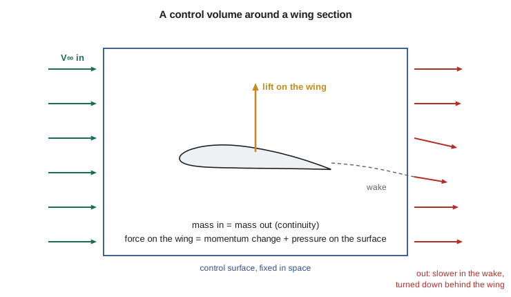
Three physical principles govern the flow: mass is conserved, Newton's second law holds for every piece of fluid, and energy is conserved. Each can be written for a control volume, a region fixed in space through which fluid passes, or for an infinitesimal fluid element. The control volume form gives powerful overall results, such as the drag of a wing from measurements in its wake. The differential form gives the detailed flow field that computer methods solve.

Conservation of mass: the continuity equation

Mass cannot be created or destroyed. For a control volume, the rate at which mass inside increases must equal the net rate at which mass flows in through the surface. Shrinking the volume to a point gives the continuity equation in differential form.

When the density is constant, the equation becomes simply \(\nabla\cdot\mathbf{V} = 0\): the velocity field must have zero divergence, so any fluid that speeds up in one direction must be fed from another. The flow is then called incompressible. Air is of course compressible, but its density changes very little when the flow speed is well below the speed of sound. The density change between the free stream and a point where the flow has been brought to rest is roughly \(M^2/2\), so at Mach 0.3 it is about 4.5 percent. The usual rule is that flows below about Mach 0.3 can be treated as incompressible. The Tern cruises near Mach 0.32, right at the edge, which is why the Block 2 team will apply a compressibility correction to its cruise numbers. That correction is a topic for AERO-310; this course treats the flow as incompressible, which is accurate for take-off, landing and the climb, where the high-lift questions are decided.

Continuity is a powerful check on any proposed velocity field. If someone hands you a formula for \(u\) and \(v\), you can verify that it could represent a real incompressible flow by testing whether \(\partial u/\partial x + \partial v/\partial y\) is zero everywhere. The program in this lesson does exactly that, numerically, for the field of a two-dimensional source, which you will meet again in Lesson 3.

Newton's second law for a fluid: Euler and Navier-Stokes

A fluid particle accelerates because forces act on it. Body forces such as gravity act on its mass; surface forces act on its boundaries. The surface forces are pressure, which always pushes normal to the surface, and viscous stresses, which arise because neighboring layers of fluid slide past one another. Writing \(\rho\,D\mathbf{V}/Dt\) equal to the sum of these forces per unit volume gives the momentum equation. For a Newtonian fluid such as air, with constant viscosity \(\mu\) and constant density, it takes the form known as the Navier-Stokes equation.

The Navier-Stokes equations, together with continuity, describe essentially every flow an aircraft meets at subsonic speed, including turbulence. Their difficulty is that the convective acceleration makes them nonlinear, and for flows at the Reynolds numbers of real aircraft the solutions contain eddies over an enormous range of sizes. Directly computing all of those eddies around a whole aircraft is still far beyond practical computing power, which is why engineers use simplified forms and models.

The most important simplification is to drop the viscous term. The result is the Euler equation, which describes an inviscid fluid. It sounds drastic, since every real fluid has viscosity, but for air flowing around a streamlined body at high Reynolds number the viscous stresses matter only in a thin boundary layer next to the surface and in the wake. Outside that layer the flow behaves almost exactly as if it were inviscid. This split, an inviscid outer flow plus a thin viscous layer, was Ludwig Prandtl's great insight in 1904, and it organizes this whole course. Lessons 2 to 9 study the inviscid outer flow, which determines lift. Lessons 10 to 12 return to the boundary layer, which determines skin-friction drag, stall and much of what high-lift devices do.

Bernoulli's equation and the pressure coefficient

Integrating the Euler equation along a streamline for steady, incompressible flow, with gravity negligible as it is for air over a wing, gives Bernoulli's equation: the static pressure plus the dynamic pressure is constant along the streamline. If the flow comes from a uniform free stream and has no vorticity, a condition explained in Lesson 2, the same constant holds everywhere in the flow.

Aerodynamicists rarely quote pressures in pascals. They use the pressure coefficient, which compares the local pressure with the free-stream pressure in units of the free-stream dynamic pressure \(q_\infty = \tfrac{1}{2}\rho V_\infty^2\). Combining its definition with Bernoulli's equation shows that, in incompressible flow, the pressure coefficient depends only on the local speed ratio.

At a stagnation point, where the flow comes to rest, \(C_p = 1\), the highest value possible in incompressible flow. Where the flow moves at free-stream speed, \(C_p = 0\). Where it moves faster, \(C_p\) is negative: suction. On a lifting wing the upper surface near the leading edge can reach \(C_p\) of minus 3 or lower, meaning the local speed is twice the free-stream speed. Because lift comes mainly from that suction, the shape of the \(C_p\) curve along the chord is the single most informative plot in airfoil design, and you will see many of them.

Similarity: the Reynolds number and the Mach number

Wind tunnel models are smaller than the aircraft and usually tested at different speeds and air densities. The results apply to the full-size aircraft only if the flows are dynamically similar. Making the Navier-Stokes equation dimensionless shows that, for an incompressible flow over geometrically similar shapes, the flow pattern depends on one number, the Reynolds number, the ratio of inertial to viscous forces. When compressibility matters, a second number, the Mach number, also enters.

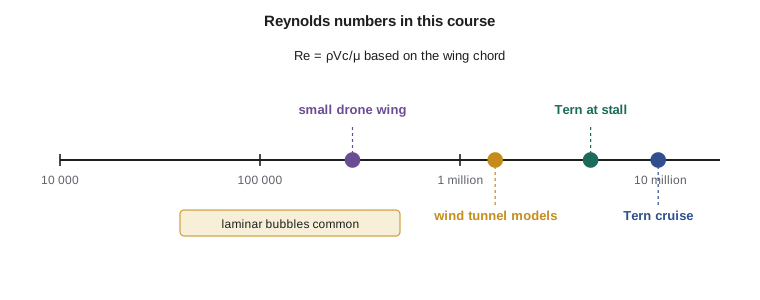
The program below computes these numbers for the cases this course keeps returning to. The Tern's wing at cruise works at a Reynolds number near 10 million on its mean chord. The same wing near the stall, slow and close to the ground, works at about 4.5 million, and its small tip chord at about 2.6 million. The Prairiewind Aerospace Skiff-W cargo drone, slow and small, flies at under 300 000. These differences are not academic. As Lesson 11 shows, a wing section can behave very differently at 300 000 than at 3 million, and the data in airfoil catalogs are always tied to a Reynolds number.

# Flow conditions for the Tern and the Skiff-W, and a numerical check of the continuity equation
import math
def isa(h):                                   # ISA troposphere: temperature, pressure, density
    T = 288.15 - 0.0065 * h
    p = 101325 * (T / 288.15) ** 5.2559
    return T, p, p / (287.05 * T)
def mu(T):                                    # Sutherland's law for the viscosity of air
    return 1.458e-6 * T ** 1.5 / (T + 110.4)
cases = [  # name, altitude m, speed m/s, reference length m
    ('Tern cruise, wing MAC', 3000, 105.6, 1.73),
    ('Tern landing stall, MAC', 0, 37.8, 1.73),
    ('Tern tip chord at stall', 0, 37.8, 1.02),
    ('Skiff-W wing chord', 0, 13.3, 0.32),
]
for name, h, V, c in cases:
    T, p, rho = isa(h)
    a = math.sqrt(1.4 * 287.05 * T)
    Re = rho * V * c / mu(T)
    q = 0.5 * rho * V ** 2
    print(f"{name:26s} Re = {Re:9.3g}  M = {V / a:.3f}  q = {q:7.0f} Pa")
# Continuity check: u = x/(x^2+y^2), v = y/(x^2+y^2) is the field of a 2D source
def vel(x, y):
    r2 = x * x + y * y
    return x / r2, y / r2
h = 1e-5
for (x, y) in [(1.0, 0.5), (-0.7, 2.0), (3.0, -1.0)]:
    dudx = (vel(x + h, y)[0] - vel(x - h, y)[0]) / (2 * h)
    dvdy = (vel(x, y + h)[1] - vel(x, y - h)[1]) / (2 * h)
    print(f"at ({x:4.1f},{y:4.1f}) du/dx + dv/dy = {dudx + dvdy: .2e}")
# Bernoulli: local pressure coefficient where the flow speeds up by 25 percent
for ratio in (0.0, 1.0, 1.25, 1.5):
    print(f"V/V_inf = {ratio:4.2f}  Cp = {1 - ratio ** 2:6.3f}")

Tern cruise, wing MAC      Re =  9.81e+06  M = 0.321  q =    5069 Pa
Tern landing stall, MAC    Re =  4.48e+06  M = 0.111  q =     875 Pa
Tern tip chord at stall    Re =  2.64e+06  M = 0.111  q =     875 Pa
Skiff-W wing chord         Re =  2.91e+05  M = 0.039  q =     108 Pa
at ( 1.0, 0.5) du/dx + dv/dy =  3.05e-11
at (-0.7, 2.0) du/dx + dv/dy = -1.39e-12
at ( 3.0,-1.0) du/dx + dv/dy =  6.94e-13
V/V_inf = 0.00  Cp =  1.000
V/V_inf = 1.00  Cp =  0.000
V/V_inf = 1.25  Cp = -0.562
V/V_inf = 1.50  Cp = -1.250

The divergence check returns values of order \(10^{-11}\) or smaller, which is round-off: the source field satisfies continuity everywhere except at the source point itself, where the formula breaks down. The last lines show how quickly suction builds: a 25 percent speed-up gives \(C_p = -0.56\), and a 50 percent speed-up gives \(-1.25\).

Testing the Block 2 wing in a wind tunnel

The Block 2 wing will be tested as a complete model in the Walter H. Beech wind tunnel at Wichita State University, a closed test section 7 ft high and 10 ft wide, about 2.1 m by 3.0 m, that has served aircraft makers in Wichita since 1948. A one-eighth-scale model, with a span of about 2.1 m and a mean chord of about 0.22 m, reaches a Reynolds number of only about 1.2 million even at 80 m/s, about 180 mph. That is roughly a quarter of the full-size value at the stall, so Tomasz's team will use the tunnel data mainly to compare design options and to study how the stall spreads along the span, and will correct the absolute lift and drag numbers for Reynolds number before they go into performance calculations.

Matching both Reynolds number and Mach number on a small model is very hard. Some research tunnels raise the Reynolds number by pressurizing the air, which raises the density, or by cooling it to cryogenic temperatures, which raises density and lowers viscosity. Commercial programs more often accept the mismatch and correct for it, using computer predictions and previous experience to bridge the gap, and confirm the result in flight test.