
ACCT-341 · Lesson 10 of 12 · 30 min
Predictive analytics: regression, forecasting and classification
Accountants make predictions constantly: budgets and forecasts, the allowance for doubtful accounts, warranty provisions, impairment tests, going concern assessments and the expectations behind analytical procedures. Predictive analytics brings statistical discipline to these judgments. This lesson introduces three workhorse techniques: regression, which explains a measure in terms of its drivers; time series forecasting, which projects a measure forward from its own history; and classification, which predicts which category an item will fall into, such as whether a customer will pay late. The aim is not to make you a statistician but to let you build simple, defensible models, judge models built by others, and understand their limits. STAT-141 covered the statistical foundations; here we apply them.
Explaining and predicting
A model can serve two purposes. An explanatory model aims to understand how drivers affect an outcome: how much does freight expense rise with each additional thousand shipments? A predictive model aims to forecast outcomes accurately, whether or not its inner workings are easy to interpret: what will next quarter's sales be? Accounting uses both. An auditor building an expectation for freight expense wants a model whose logic can be explained and documented. A treasury team forecasting cash wants accuracy above all. In both cases, the model must be tested against data it was not built on, because a model can fit the past perfectly and still predict the future badly.
Regression
Linear regression estimates the relationship between an outcome and one or more drivers by fitting the line, or with several drivers the plane, that minimizes the sum of squared differences between actual and fitted values. This is ordinary least squares (OLS). Each coefficient estimates how much the outcome changes for a one-unit change in that driver, holding the others constant. The fitted equation has the form below, where y is the outcome, the x terms are the drivers, the b terms are the estimated coefficients and e is the residual, the part the model does not explain.
Cedarbrook's freight expense should depend mainly on how many shipments it makes and on fuel prices, which carriers pass on as surcharges. Maya regresses 24 months of freight expense on shipments and a fuel price index, then looks for months where actual freight differs from what the model expects.
# Explaining monthly freight expense with shipments and a fuel index
import numpy as np
shipments = np.array([3120, 2980, 3410, 3890, 4420, 4710, 4650, 4580, 4300,
                      3950, 3380, 3050, 3200, 3090, 3520, 4010, 4560, 4840,
                      4790, 4700, 4410, 4060, 3460, 3140])        # 2024-2025
fuel = np.array([100, 101, 103, 104, 106, 108, 107, 105, 104, 102, 101, 100,
                 99, 100, 102, 105, 107, 109, 110, 108, 106, 104, 103, 102])
freight = np.array([181, 175, 199, 228, 262, 282, 277, 270, 252, 230, 197,
                    178, 185, 179, 205, 236, 270, 291, 290, 283, 264, 241,
                    203, 213])                                    # $ thousands
X = np.column_stack([np.ones(24), shipments, fuel])
coef, *_ = np.linalg.lstsq(X, freight, rcond=None)
fitted = X @ coef
resid = freight - fitted
r2 = 1 - (resid ** 2).sum() / ((freight - freight.mean()) ** 2).sum()
se = np.sqrt((resid ** 2).sum() / (24 - 3))
print(f"freight = {coef[0]:.1f} + {coef[1]*1000:.1f} per 1,000 shipments"
      f" + {coef[2]:.2f} per fuel index point")
print(f"R-squared {r2:.3f}, residual standard error {se:.1f}")
for i in np.argsort(-np.abs(resid))[:2]:
    yr, mo = 2024 + i // 12, i % 12 + 1
    print(f"{yr}-{mo:02d}: actual {freight[i]}, expected {fitted[i]:.1f},"
f" difference {resid[i]:+.1f} ({resid[i] / se:+.1f} standard errors)")freight = -251.9 + 47.9 per 1,000 shipments + 2.86 per fuel index point R-squared 0.981, residual standard error 5.8 2025-12: actual 213, expected 189.6, difference +23.4 (+4.0 standard errors) 2024-03: actual 199, expected 205.4, difference -6.4 (-1.1 standard errors)
The model fits closely: shipments and fuel together explain 98 percent of the month-to-month variation in freight, as measured by R-squared. Each additional thousand shipments adds about 47,900 dollars of freight, and each point on the fuel index adds about 2,860. The negative intercept has no business meaning; it is simply where the fitted plane crosses zero, far outside the range of the data, and it is a reminder never to use a regression to predict outside the range it was fitted on. The useful output is the residual analysis. December 2025 freight was 213 thousand, about 23 thousand more than the model expects, four standard errors above it. No other month is more than about one standard error away. Something unusual happened in December: perhaps a duplicate carrier invoice, a year-end accrual estimated too high, or a freight cost misclassified from another account. Maya now knows exactly where to look.
This is how regression supports analytical procedures in audit: the model builds an independent expectation from non-financial drivers, and the difference between expectation and recorded amount directs further work. One refinement would improve this model. The December 2025 outlier was included in the data used to fit the model, which pulls the fitted line toward it and inflates the standard error. A cleaner approach fits the model on 2024 and the first eleven months of 2025, then predicts December. Lesson 11 returns to this.
| Check | Why it matters | What to look for |
|---|---|---|
| Plausible signs and sizes | Coefficients should make business sense | Freight should rise, not fall, with shipments |
| Fit (R-squared, residual standard error) | How much variation the model explains and how precise it is | High R-squared alone is not proof of a good model |
| Residual pattern | Systematic patterns suggest missing drivers | Residuals that trend or repeat seasonally |
| Range of the data | Predictions outside the range are unreliable | Do not extrapolate far beyond the fitted range |
| Correlated drivers (multicollinearity) | Highly correlated drivers make coefficients unstable | Coefficients that change sign when a driver is added |
| Out-of-sample performance | The real test of a predictive model | Errors on data not used to fit the model |
Forecasting time series
A time series is a measure recorded at regular intervals, such as monthly sales. Most business time series combine a trend, a repeating seasonal pattern and irregular noise. Cedarbrook's sales follow the construction season, peaking in early summer and falling in winter, on a gently rising trend. Forecasting methods range from simple to sophisticated, and simple methods are often surprisingly hard to beat.
| Method | How it works | Strengths and limits |
|---|---|---|
| Naive | Next period equals this period | A baseline; ignores seasonality |
| Seasonal naive | Next period equals the same period last year | Captures seasonality; ignores growth |
| Moving average | Average of the last several periods | Smooths noise; lags behind trends |
| Growth-adjusted seasonal | Same period last year times recent growth | Simple, explainable; assumes growth continues |
| Regression with trend and seasonal terms | Fits a trend plus an adjustment for each month | Explainable; assumes a stable pattern |
| Exponential smoothing (ETS) | Weights recent observations more heavily; can model trend and season | Widely used; built into Excel as FORECAST.ETS |
| ARIMA and machine learning methods | Model complex patterns and many drivers | Need more data and expertise; harder to explain |
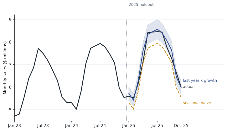
The right way to choose among methods is to test them on a holdout: fit each method on earlier data, forecast a period you already know, and compare the forecasts with what actually happened. A common accuracy measure is the mean absolute percentage error (MAPE), the average of the absolute forecast errors expressed as a percentage of actual values. The program below uses simulated monthly sales for 2023 to 2025, fits three methods on 2023 and 2024, and compares their forecasts of 2025.
# Forecasting monthly sales: compare three methods on a 2025 holdout
import numpy as np
rng = np.random.default_rng(41)
months = np.arange(36)                                  # Jan 2023 to Dec 2025
season = np.array([0.80, 0.78, 0.90, 1.02, 1.14, 1.20,
                   1.19, 1.17, 1.10, 1.02, 0.88, 0.80])
sales = (6.08 + 0.034 * months) * season[months % 12] \
        * rng.normal(1, 0.025, 36)                      # $ millions
train, test = sales[:24], sales[24:]
naive = train[-12:]                                     # same month last year
growth = train[12:].sum() / train[:12].sum()
seasonal_growth = train[-12:] * growth                  # last year x growth
t = months[:24]
X = np.column_stack([np.ones(24), t] + [(t % 12 == m) * 1.0 for m in range(1, 12)])
b, *_ = np.linalg.lstsq(X, np.log(train), rcond=None)
tt = months[24:]
Xf = np.column_stack([np.ones(12), tt] + [(tt % 12 == m) * 1.0 for m in range(1, 12)])
regression = np.exp(Xf @ b)
def mape(f):
    return np.mean(np.abs(test - f) / test) * 100
for name, f in [("seasonal naive", naive), ("last year x growth", seasonal_growth),
                ("trend + season regression", regression)]:
    print(f"{name:<27} 2025 total {f.sum():6.2f}   MAPE {mape(f):4.1f}%")
print(f"{'actual':<27} 2025 total {test.sum():6.2f}")seasonal naive 2025 total 80.51 MAPE 6.2% last year x growth 2025 total 86.92 MAPE 2.3% trend + season regression 2025 total 86.89 MAPE 2.4% actual 2025 total 85.80
The seasonal naive forecast, which simply repeats 2024, misses the growth and undershoots by over 5 million, with an average monthly error of 6.2 percent. Both methods that account for growth do much better, with errors of about 2.3 to 2.4 percent and annual totals within about 1.1 million of the actual 85.8 million. The simple growth-adjusted method is as accurate as the regression and easier to explain. That is a common result: complexity should earn its place by improving accuracy on holdout data, not be assumed to help.
Every forecast is uncertain, and a single number hides that. Good practice presents a range, such as a forecast of 89 million with an 80 percent prediction interval of 86 to 92 million, and explains the main assumptions, such as continued growth in the West contract. Forecasts used in financial reporting, for example in impairment tests or going concern assessments, also need documented assumptions that can be compared with history and challenged by auditors. A useful check is to compare past forecasts with actual outcomes: a company whose forecasts have been consistently optimistic should adjust its process, and an auditor should be more skeptical of its current forecasts.
Classification
Classification predicts which of two or more categories an item belongs to. Accounting examples include whether a customer will pay more than 60 days late, whether an expense claim breaches policy, whether a journal entry is likely to be erroneous, and whether a vendor invoice is a duplicate. Logistic regression is a standard starting point for two-category problems. It estimates the probability of the event from the drivers, using an S-shaped function that keeps probabilities between 0 and 1, and its coefficients show which drivers raise or lower the probability.
Cedarbrook's credit team wants to know which customers are likely to pay late so it can call them before invoices fall overdue. The program below simulates 3,000 customers with four drivers: average days to pay last year, credit utilization (balance divided by credit limit), years as a customer and disputed invoices. It fits a logistic regression on 70 percent of customers and evaluates it on the other 30 percent.
# Which customers are likely to pay more than 60 days late? (simulated)
import numpy as np
from sklearn.linear_model import LogisticRegression
from sklearn.model_selection import train_test_split
rng = np.random.default_rng(12)
n = 3000
avg_days = rng.gamma(4, 9, n)                  # average days to pay last year
utilization = rng.uniform(0, 1.3, n)           # balance / credit limit
years = rng.integers(0, 25, n)                 # years as a customer
disputes = rng.poisson(0.4, n)                 # disputed invoices last year
z = -6.0 + 0.06 * avg_days + 1.8 * utilization - 0.05 * years + 0.5 * disputes
late = rng.random(n) < 1 / (1 + np.exp(-z))
X = np.column_stack([avg_days, utilization, years, disputes])
X_tr, X_te, y_tr, y_te = train_test_split(X, late, test_size=0.3,
                                          random_state=1, stratify=late)
model = LogisticRegression(max_iter=1000).fit(X_tr, y_tr)
print("late payers in test set:", y_te.sum(), "of", len(y_te))
names = ["avg days to pay", "utilization", "years as customer", "disputes"]
for nm, c in zip(names, model.coef_[0]):
    print(f"  {nm:<18} coefficient {c:+.3f}")
p = model.predict_proba(X_te)[:, 1]
for cut in (0.5, 0.2):
    flag = p >= cut
    tp = (flag & y_te).sum(); fp = (flag & ~y_te).sum(); fn = (~flag & y_te).sum()
    print(f"threshold {cut}: flagged {flag.sum()}, caught {tp}, "
          f"false alarms {fp}, missed {fn}, "
f"precision {tp / flag.sum():.2f}, recall {tp / (tp + fn):.2f}")late payers in test set: 75 of 900 avg days to pay coefficient +0.060 utilization coefficient +1.622 years as customer coefficient -0.060 disputes coefficient +0.545 threshold 0.5: flagged 19, caught 12, false alarms 7, missed 63, precision 0.63, recall 0.16 threshold 0.2: flagged 96, caught 36, false alarms 60, missed 39, precision 0.38, recall 0.48
The coefficients have sensible signs: slower past payment, higher utilization and more disputes raise the probability of late payment, while longer relationships lower it. The evaluation shows the central trade-off in classification. Only 75 of the 900 test customers paid late, a base rate of about 8 percent. At the conventional threshold of 0.5, the model flags just 19 customers; 12 of them do pay late, a precision of 0.63, but it misses 63 of the 75 late payers, a recall of only 0.16. Lowering the threshold to 0.2 flags 96 customers and catches 36 late payers, nearly half, at the cost of 60 false alarms.
| Measure | Definition | Question it answers |
|---|---|---|
| Precision | True positives ÷ all flagged | When the model flags a customer, how often is it right? |
| Recall (sensitivity) | True positives ÷ all actual positives | What share of late payers does the model catch? |
| False positive | Flagged but not actually late | Cost: an unnecessary call |
| False negative | Not flagged but actually late | Cost: a late payment that might have been prevented |
| Base rate | Share of items that are actually positive | How rare is the event? Rare events make precision hard |
Which threshold is right depends on the costs of each kind of error, which is a business judgment, not a statistical one. If a reminder call costs a few dollars and a late payment costs much more in financing and collection effort, the credit team should accept many false alarms to catch more late payers, and the lower threshold is better. If each flag triggered a credit hold that might lose a good customer, a higher threshold would be wiser. Accuracy, the share of all predictions that are correct, is a poor guide for rare events: a model that predicted nobody would pay late would be 92 percent accurate and completely useless.
Worked problem
Choosing a threshold
Each reminder call costs Cedarbrook about 15 dollars of staff time. Each late payment that a call would have prevented saves about 120 dollars in financing and collection costs, and calls prevent about half of the late payments they target. Using the test results, which threshold is better?
Show solution
- At 0.5: 19 calls cost 285 dollars; 12 late payers called, about 6 prevented, saving about 720 dollars. Net benefit about 435 dollars.
- At 0.2: 96 calls cost 1,440 dollars; 36 late payers called, about 18 prevented, saving about 2,160 dollars. Net benefit about 720 dollars.
- The lower threshold yields a larger net benefit despite more false alarms.
- The analysis should be repeated with real cost estimates and monitored after the change.
Answer: The 0.2 threshold, because the benefit of catching more late payers outweighs the cost of extra calls.
Overfitting and model risk
Overfitting happens when a model learns the noise in its training data rather than the underlying pattern. An overfitted model looks excellent on the data it was built on and performs poorly on new data. The defenses are to keep models as simple as the problem allows, to evaluate on holdout data or with cross-validation, and to be suspicious of results that seem too good. A forecast with a MAPE of 0.1 percent on its own training data proves nothing.
Models used in decisions also carry broader risks: errors in data or code, inappropriate use outside the conditions they were built for, drift as the business changes, and bias. A credit model trained on historical decisions can perpetuate past unfairness, and models used for consumer credit decisions are subject to federal fair lending rules, while personal information raises obligations under state privacy laws, which lesson 12 discusses. Good practice includes documenting each model's purpose, data, assumptions and limitations, having someone independent review it, monitoring its performance over time, and keeping a human accountable for decisions.
Beyond the supervised methods in this lesson, which learn from examples with known outcomes, there are unsupervised methods that find structure without labeled outcomes. Clustering groups similar items, such as customers with similar buying patterns, and anomaly detection identifies items unlike the rest, such as unusual journal entries or payments. Lesson 11 applies some of these ideas to audit.
Tools
Excel offers regression through the Analysis ToolPak and the LINEST function, and forecasting through FORECAST.LINEAR, FORECAST.ETS and the Forecast Sheet command, which produces a forecast with a prediction interval in a few clicks. Power BI and Tableau include forecasting features in their line charts. Python's numpy, statsmodels and scikit-learn libraries, used here, handle everything from simple regression to complex machine learning. Whatever the tool, the discipline is the same: define the question, test on holdout data, check the residuals, communicate the uncertainty and document the model.
Common mistakes
MistakeJudging a model by how well it fits the data it was built on.
InsteadTest on holdout data the model has not seen.
MistakeExtrapolating a regression far outside the fitted range.
InsteadUse regression only within, or close to, the range of the data.
MistakePresenting a forecast as a single certain number.
InsteadShow a range and state the key assumptions.
MistakeUsing accuracy to evaluate a model for a rare event.
InsteadUse precision, recall and the costs of each error.
MistakeAssuming a more complex model is better.
InsteadLet holdout accuracy decide; simple models are easier to explain and often as accurate.
Summary and key terms
- Explanatory models show how drivers affect outcomes; predictive models aim for accuracy on new data.
- OLS regression estimates coefficients for each driver; check signs, fit, residuals, range and out-of-sample performance.
- Residuals from a driver-based model identify unusual periods, such as Cedarbrook's December 2025 freight.
- Time series combine trend, seasonality and noise; simple growth-adjusted seasonal methods are often hard to beat.
- Choose forecasting methods by holdout accuracy, such as MAPE, and present forecasts with ranges.
- Logistic regression estimates the probability of a category, such as late payment.
- Precision and recall trade off as the threshold moves; choose it from the costs of each error.
- Guard against overfitting and manage model risk with documentation, review, monitoring and human accountability.
- Regression
- A method for estimating the relationship between an outcome and one or more drivers.
- Coefficient
- The estimated change in the outcome for a one-unit change in a driver, others held constant.
- R-squared
- The share of variation in the outcome explained by the model.
- Residual
- The difference between an actual value and the model's fitted value.
- Holdout
- Data withheld from model fitting and used to test predictions.
- MAPE
- Mean absolute percentage error, a measure of forecast accuracy.
- Logistic regression
- A model estimating the probability that an item belongs to a category.
- Precision
- The share of flagged items that are truly positive.
- Recall
- The share of truly positive items that the model flags.
- Overfitting
- Fitting noise in the training data so that predictions on new data are poor.
Practice problems
Work each problem on paper first, then reveal the answer to check.
In the regression program, how much does freight rise for each additional thousand shipments?
Show answer
About 47,900 dollars.
Why should the negative intercept not be interpreted?
Show answer
Zero shipments and a zero fuel index are far outside the data; the intercept only positions the fitted plane.
Give two possible explanations for December 2025's freight residual.
Show answer
A duplicate carrier invoice, an overestimated accrual, or a misclassified cost.
How could the regression be improved so the outlier does not affect the expectation?
Show answer
Fit on data excluding December 2025, then predict December.
In the forecasting program, which method had the highest MAPE and why?
Show answer
Seasonal naive, at 6.2 percent, because it ignores growth.
A forecast of 30 against an actual of 25 and a forecast of 18 against an actual of 20. What is the MAPE?
Show answer
(20% + 10%) ÷ 2 = 15 percent.
In the classification program, what are precision and recall at the 0.2 threshold?
Show answer
0.38 and 0.48.
Why is accuracy misleading for predicting late payment here?
Show answer
Only about 8 percent pay late, so predicting no one is late would be 92 percent accurate and useless.
Change the threshold in the classification program to 0.1. What would you expect?
Show answer
More customers flagged, higher recall, lower precision.
Name two practices for managing model risk.
Show answer
Documentation, independent review, performance monitoring, and human accountability for decisions.
Lesson quiz · 5 questions
Score 60% or more to complete this lesson.
Create a free account to save your progress, take quizzes and earn a certificate.