
ROB-230 · Lesson 7 of 12 · 31 min
Frequency response and Bode plots
Feed a sinusoid into a stable LTI system and, once the transients die away, a sinusoid comes out at exactly the same frequency, changed only in amplitude and phase. How the amplitude ratio and phase shift vary with frequency is the system's frequency response, and it is one of the most useful descriptions an engineer has. It can be measured directly on hardware with a signal generator or a chirp, without knowing any equations. It shows at a glance which frequencies a sensor passes, where a mechanism resonates, how much noise a filter removes and, through gain and phase margins, how close a feedback loop is to instability. The standard way to draw it is the Bode plot, with logarithmic frequency and gain in decibels, on which complicated systems become sums of simple straight-line pieces. This lesson derives the frequency response from the transfer function, teaches the asymptotic sketching rules, and applies them to bandwidth, resonance and stability margins.
Sinusoids in, sinusoids out
Lesson 2 noted that complex exponentials pass through LTI systems unchanged in shape. Here is why. If the input is \( x(t) = e^{j\omega t} \), convolution with the impulse response gives
The integral is just the transfer function evaluated on the imaginary axis, \( s = j\omega \). For a real sinusoid \( A\cos\omega t \), taking real parts gives the steady-state output
The magnitude \( |G(j\omega)| \) is the gain at that frequency, and the angle \( \angle G(j\omega) \) is the phase shift; a negative phase means the output lags the input. Together they form the frequency response. For a stable system it can be measured by injecting sinusoids of increasing frequency, or a swept sine (chirp), or broadband noise followed by spectral analysis (lesson 8), and comparing output with input. Robot engineers routinely measure the frequency response of servo axes this way to find resonances before tuning.
Worked problem
Response of a first-order sensor to a vibration
A force sensor behaves as \( G(s) = 1/(0.01s + 1) \). The true force oscillates as \( 5\cos(100t) \) N. What does the sensor read in steady state?
Show solution
- \( G(j100) = 1/(1 + j \times 0.01 \times 100) = 1/(1 + j) \).
- Magnitude \( 1/\sqrt{2} = 0.707 \); phase \( -\arctan(1) = -45° \).
- Reading: \( 5 \times 0.707\cos(100t - 45°) = 3.54\cos(100t - 0.785) \) N.
Answer: The sensor reports an oscillation of only 3.54 N, lagging by 45°, which is 7.9 ms at 100 rad/s. At this frequency, the sensor's corner frequency, it underestimates the force amplitude by 29 %.
Decibels and the Bode plot
Gains in robotics span many orders of magnitude, from the near-unity gain of a sensor at low frequency to the tiny gain of a filter in its stopband, so they are expressed in decibels:
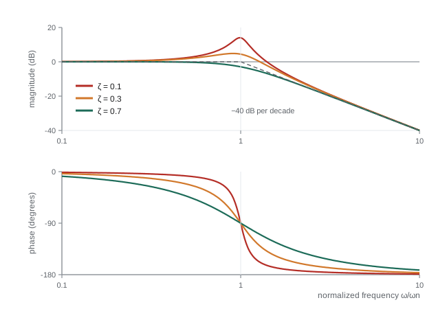
A gain of 10 is +20 dB, 100 is +40 dB, 1 is 0 dB, 0.1 is −20 dB, and \( 1/\sqrt{2} \) is −3 dB. Decibels turn multiplication into addition: the dB gain of blocks in series is the sum of their dB gains, and the phases also add. A Bode plot draws magnitude in dB and phase in degrees against frequency on a logarithmic axis. A factor of ten in frequency is a decade, and a factor of two an octave. On these axes most transfer-function factors become straight lines, so a complicated response can be sketched by adding a few simple pieces, which is why Hendrik Bode's 1940 invention is still used daily.
Sketching rules for the basic factors
Any rational transfer function factors into a gain, poles and zeros at the origin, real poles and zeros, and complex pairs. Each has a simple Bode shape.
- Constant gain K: a flat line at \( 20\log_{10}K \) dB, phase 0° (or −180° if K is negative).
- Integrator 1/s: a straight line falling at −20 dB per decade, passing 0 dB at ω = 1 rad/s, with a constant phase of −90°. A differentiator s rises at +20 dB per decade with +90°.
- Real pole \( 1/(s/\omega_c + 1) \): flat at 0 dB below the corner frequency \( \omega_c \), falling at −20 dB per decade above it. The true curve is 3 dB below the corner of the asymptotes at \( \omega_c \). The phase goes from 0° to −90°, passing −45° at \( \omega_c \), and changes mostly between \( \omega_c/10 \) and \( 10\omega_c \).
- Real zero \( s/\omega_c + 1 \): the mirror image, rising at +20 dB per decade with phase going to +90°.
- Complex pole pair (second-order, \( \omega_n \), \( \zeta \)): flat at 0 dB, then falling at −40 dB per decade above \( \omega_n \), with phase from 0° to −180° passing −90° at \( \omega_n \). For \( \zeta < 0.707 \) there is a resonant peak near \( \omega_n \) of height about \( 1/(2\zeta) \), or \( -20\log_{10}(2\zeta) \) dB, and the phase changes sharply. At \( \zeta = 0.1 \) the peak is +14 dB, a fivefold amplification.
- Pure delay \( e^{-sT} \): magnitude exactly 0 dB at all frequencies but phase \( -\omega T \) radians, growing without limit. This is why delay is so damaging to feedback loops.
Worked problem
Sketching a Bode plot
Sketch the magnitude of \( G(s) = \dfrac{100}{s(s/10 + 1)} \), a motor position plant with integrator, and find where it crosses 0 dB.
Show solution
- At low frequency the integrator dominates: \( |G| \approx 100/\omega \), a −20 dB/decade line through 40 dB at ω = 1 rad/s.
- At the corner ω = 10 rad/s the pole adds another −20 dB/decade; the asymptote there is \( 100/10 = 10 \), i.e. 20 dB.
- Above 10 rad/s the slope is −40 dB/decade: \( |G| \approx 1000/\omega^2 \), which reaches 0 dB at \( \omega = \sqrt{1000} = 31.6 \) rad/s.
- Exact check: \( |G(j31.6)| = 100/(31.6\sqrt{1 + 10}) = 100/(31.6 \times 3.317) = 0.954 \), so the true crossover is a little lower, about 30.8 rad/s.
Answer: The magnitude falls at −20 dB/decade to 20 dB at 10 rad/s, then at −40 dB/decade, crossing 0 dB at about 31 rad/s. The asymptotes give the answer within a few per cent with no calculator, which is the point of the method.
Bandwidth and resonance
Bandwidth measures how fast a system can respond. For a low-pass system, the bandwidth \( \omega_B \) is the frequency at which the gain has fallen 3 dB below its low-frequency value: signals below it pass largely unchanged; signals above it are attenuated. For a first-order system the bandwidth equals \( 1/\tau \), and rise time and bandwidth are linked by the useful rule \( t_r \approx 2.2/\omega_B = 0.35/f_B \). A sensor with 100 Hz bandwidth cannot faithfully report events shorter than a few milliseconds; a joint servo with 10 Hz closed-loop bandwidth cannot track trajectories containing motion much faster than 10 Hz. Specifications for robot actuators and sensors therefore quote bandwidth constantly.
Resonance is the opposite danger: a lightly damped mode amplifies inputs near its natural frequency. A robot arm whose first structural mode is at 15 Hz will shake violently if the controller or the trajectory excites 15 Hz, which is why trajectory planners avoid exciting known modes and why notch filters (lesson 11) are inserted in servo loops to remove them.
Worked problem
Bandwidth of a closed-loop joint
A joint's closed-loop transfer function is \( T(s) = 400/(s^2 + 28s + 400) \). Find \( \omega_n \), \( \zeta \), whether there is a resonant peak, and estimate the bandwidth.
Show solution
- \( \omega_n = 20 \) rad/s; \( \zeta = 28/40 = 0.7 \).
- At ζ = 0.7 the resonant peak just disappears, so the response is flat and then rolls off.
- For a second-order system \( \omega_B = \omega_n\sqrt{1 - 2\zeta^2 + \sqrt{2 - 4\zeta^2 + 4\zeta^4}} \). With ζ = 0.7: \( 1 - 0.98 + \sqrt{2 - 1.96 + 0.9604} = 0.02 + 1.0002 = 1.0202 \), so \( \omega_B = 20 \times 1.010 = 20.2 \) rad/s.
Answer: With ζ = 0.7, the bandwidth is almost exactly \( \omega_n \), about 20 rad/s (3.2 Hz), and there is no resonant peak. The joint can track commands containing frequencies up to roughly 3 Hz.
Stability margins
Lesson 6 showed that a loop goes unstable when the signal returning around the loop comes back with enough gain and the wrong phase. On the Bode plot of the loop transfer function L(jω), this is easy to see. The gain crossover frequency \( \omega_{gc} \) is where \( |L| = 1 \) (0 dB). The phase crossover frequency \( \omega_{pc} \) is where \( \angle L = -180° \). Two numbers measure how far the loop is from instability:
- Phase margin: \( PM = 180° + \angle L(j\omega_{gc}) \), the extra phase lag that would make the loop unstable. Typical designs aim for 45° to 60°. Phase margin relates closely to damping: roughly \( \zeta \approx PM/100 \) for PM up to about 60°.
- Gain margin: \( GM = -20\log_{10}|L(j\omega_{pc})| \) dB, the extra gain that would make the loop unstable. Typical designs aim for at least 6 dB, a factor of two.
These margins come from the Nyquist stability criterion, which ROB-300 covers in full. For most robot servo loops, where L is stable and has a single gain crossover, the simple rule is: the closed loop is stable if the phase margin and gain margin are both positive.
Worked problem
Delay and phase margin
The integrator loop of lesson 6 is \( L(s) = K\,e^{-0.05s}/s \). Find the phase margin for K = 15 and the gain K at which the loop becomes unstable.
Show solution
- |L| = K/ω, so the gain crossover is \( \omega_{gc} = K \).
- Phase: \( -90° - \omega \times 0.05 \times 180/\pi \).
- K = 15: phase at 15 rad/s is \( -90° - 0.75 \text{ rad} = -90° - 43.0° = -133.0° \), so PM = 47.0°.
- Instability when the phase at crossover reaches −180°: \( 0.05K = \pi/2 \), so \( K = 31.4 \) s⁻¹.
Answer: At K = 15 the phase margin is 47°, comfortably stable, matching the modest overshoot seen in lesson 6. At K ≈ 31 the margin vanishes, exactly where the simulation began to oscillate without decaying. The delay's magnitude is harmless; its phase is what limits the gain.
import numpy as np
w = np.logspace(-1, 3, 4001)           # 0.1 to 1000 rad/s
s = 1j*w
for K in [100, 20]:
    L = K/(s*(s/10 + 1)) * np.exp(-0.01*s)   # motor plant plus 10 ms delay
    mag = 20*np.log10(np.abs(L))
    ph = np.degrees(np.unwrap(np.angle(L)))
    i = np.argmin(np.abs(mag))               # gain crossover
    j = np.argmin(np.abs(ph + 180))          # phase crossover
print(f"K = {K:3d}: crossover {w[i]:5.1f} rad/s, phase margin {180 + ph[i]:5.1f} deg, gain margin {-mag[j]:5.1f} dB")K = 100: crossover 30.8 rad/s, phase margin 0.3 deg, gain margin 0.1 dB K = 20: crossover 12.5 rad/s, phase margin 31.5 deg, gain margin 14.1 dB
The script evaluates L(jω) on a fine logarithmic grid, finds the crossovers numerically and reports the margins. With K = 100, the plant sketched earlier plus a 10 ms delay, both margins are essentially zero: the loop sits on the edge of instability and would oscillate. Cutting the gain by a factor of five lowers the crossover frequency, where the plant and delay contribute less phase lag, and gives about 31° of phase margin and 14 dB of gain margin. That is stable but still short of the 45° target, so the response would overshoot noticeably; lead compensation, in ROB-300, recovers phase margin without giving up so much speed.
| Factor | Magnitude slope | Phase | Key point |
|---|---|---|---|
| Gain K | 0 dB/decade | 0° | Level 20 log K |
| Integrator 1/s | −20 dB/decade | −90° | Passes 0 dB at 1 rad/s |
| Real pole | 0, then −20 dB/decade | 0° to −90° | −3 dB and −45° at the corner |
| Real zero | 0, then +20 dB/decade | 0° to +90° | +3 dB and +45° at the corner |
| Complex pole pair | 0, then −40 dB/decade | 0° to −180° | Peak about −20 log(2ζ) dB if ζ < 0.707 |
| Delay \( e^{-sT} \) | 0 dB/decade | \( -\omega T \), unbounded | Erodes phase margin |
Common mistakes
MistakeUsing 10 log₁₀ for amplitude ratios
InsteadAmplitude (voltage, displacement) ratios use 20 log₁₀; 10 log₁₀ is for power ratios.
MistakeForgetting the 3 dB correction at a real corner
InsteadThe true curve is 3 dB below the asymptote corner and 1 dB below an octave either side.
MistakeIgnoring delay because it does not change magnitude
InsteadDelay adds phase lag that grows with frequency and reduces phase margin.
MistakeApplying frequency response to an unstable system
InsteadSteady-state sinusoidal response exists only for stable systems; for loops, analyse L(jω) and use margins.
MistakeConfusing hertz and radians per second on a Bode axis
InsteadLabel the axis and convert with ω = 2πf before applying formulas.
Summary and key terms
- A stable LTI system responds to a sinusoid with a sinusoid of the same frequency, scaled by |G(jω)| and shifted by ∠G(jω).
- The frequency response is the transfer function evaluated at s = jω and can be measured directly on hardware.
- Bode plots use decibels and logarithmic frequency, so factors in series add.
- Real poles roll off at −20 dB/decade, complex pairs at −40 dB/decade with a resonant peak if lightly damped, and delay adds unbounded phase lag.
- Bandwidth is the −3 dB frequency and sets how fast a system can respond; rise time is about 0.35/f_B.
- Phase margin and gain margin measure a loop's distance from instability; aim for 45° to 60° and at least 6 dB.
- Delay limits achievable loop gain through its phase lag.
- Frequency response
- The gain and phase of a system as functions of frequency, G(jω).
- Decibel
- A logarithmic unit of gain, 20 log₁₀ of an amplitude ratio.
- Bode plot
- Plots of magnitude in dB and phase against logarithmic frequency.
- Corner frequency
- The frequency at which a pole or zero asymptote changes slope.
- Decade
- A tenfold change in frequency.
- Bandwidth
- The frequency at which gain falls 3 dB below its low-frequency value.
- Resonant peak
- A maximum in the magnitude response of a lightly damped system near its natural frequency.
- Gain crossover frequency
- The frequency where the loop gain is 0 dB.
- Phase margin
- Additional phase lag at gain crossover that would cause instability.
- Gain margin
- Additional gain at phase crossover that would cause instability.
Practice problems
Work each problem on paper first, then reveal the answer to check.
Express gains of 1,000 and 0.01 in decibels.
Show answer
+60 dB and −40 dB.
What is the gain and phase of 1/(s + 1) at ω = 1 rad/s?
Show answer
0.707 (−3 dB) and −45°.
A first-order sensor has τ = 2 ms. What is its bandwidth in hertz?
Show answer
\( 1/(2\pi \times 0.002) = 79.6 \) Hz.
Estimate the rise time of a system with 5 Hz bandwidth.
Show answer
About 0.35/5 = 70 ms.
What is the resonant peak in dB for ζ = 0.05?
Show answer
About \( -20\log_{10}(0.1) = 20 \) dB.
What phase lag does a 20 ms delay add at 50 rad/s?
Show answer
1 rad, 57.3°.
A loop has phase −150° at gain crossover. What is its phase margin?
Show answer
30°.
A loop has |L| = 0.25 at phase crossover. What is its gain margin?
Show answer
+12 dB.
At high frequency, what slope does \( 1/(s(s + 5)(s + 20)) \) have?
Show answer
−60 dB/decade.
Two blocks of 12 dB and −5 dB are in series. What is the total gain in dB?
Show answer
7 dB.
Lesson quiz · 5 questions
Score 60% or more to complete this lesson.
Create a free account to save your progress, take quizzes and earn a certificate.