
ROB-230 · Lesson 11 of 12 · 30 min
Digital filters for robot sensors
Raw sensor data are rarely fit to use directly. Encoder velocity estimates are noisy, IMU readings carry vibration from motors and propellers, force sensors pick up structural ringing, and current measurements ripple at the PWM frequency. Digital filters clean these signals inside the controller, and choosing and implementing them well is one of the most practical skills in robotics. Every filter, however, is a trade: it removes some frequencies and inevitably delays or distorts others, and delay inside a feedback loop costs phase margin, as lessons 6, 7 and 9 showed. This lesson builds on the difference equations and z-transforms of lesson 10 to design the filters roboticists use every day: moving averages, first- and second-order IIR low-pass filters, high-pass filters, notch filters for motor and structural resonances, and differentiating filters for velocity. It compares FIR and IIR designs, explains group delay, and finishes with implementation advice for embedded code.
Specifying a filter
A filter is specified by what it should pass and what it should block. A low-pass filter passes frequencies below a cutoff and attenuates those above; a high-pass filter does the reverse; a band-pass filter passes a range; a band-stop or notch filter removes a narrow range. On a magnitude plot, the passband is where gain should stay near 1, the stopband is where gain must be small, and the transition band lies between. The steeper the transition, the higher the filter order needed and the more delay the filter adds. Specifications also cover phase: whether a constant delay is acceptable, and how much delay the control loop can tolerate. For control loops, delay is usually the binding constraint; for logged data processed offline, sharpness can be bought freely.
FIR filters: moving averages and beyond
An FIR filter computes a weighted sum of the last N inputs, \( y[n] = \sum_{k=0}^{N-1} h[k]x[n-k] \). The moving average, with all weights equal to 1/N, is the simplest. Its frequency response is
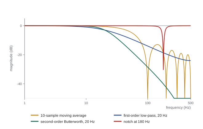
which has zeros at multiples of \( f_s/N \): a moving average over exactly one period of an interference frequency removes it completely. Averaging 20 samples at 1 kHz nulls 50 Hz and all its harmonics; averaging 50 samples at 3 kHz nulls 60 Hz and its harmonics. Its sidelobes are high, so it is a poor general low-pass filter, but it is excellent for white noise, which it reduces by \( \sqrt{N} \), and for removing a known periodic disturbance.
FIR filters with symmetric coefficients have linear phase: every frequency is delayed by the same amount, \( (N-1)/2 \) samples, so waveform shapes are preserved. They are always stable, because there is no feedback. Their drawback is length: a sharp FIR low-pass filter may need dozens or hundreds of taps, and its delay grows with its length. Windowed-sinc and least-squares methods design such filters; libraries such as SciPy provide them.
Worked problem
Moving average for a known interference
A force sensor sampled at 2 kHz has interference at 100 Hz from a nearby motor drive. What moving-average length removes it, and what delay does that filter add?
Show solution
- Nulls occur at multiples of \( f_s/N \). Choose \( f_s/N = 100 \) Hz, so N = 20.
- Delay \( (N - 1)/2 = 9.5 \) samples \( = 9.5/2000 = 4.75 \) ms.
- The filter also nulls 200, 300 Hz and so on, and reduces white noise by \( \sqrt{20} = 4.5 \).
Answer: A 20-sample moving average removes the 100 Hz interference and its harmonics at the cost of 4.75 ms of delay. For a slow force-limit check that is acceptable; inside a fast force-control loop, a notch filter would remove the interference with far less delay.
IIR low-pass filters
IIR filters achieve a given sharpness with far fewer coefficients, and far less delay, than FIR filters, by feeding back past outputs. The first-order low-pass filter,
is the workhorse of embedded robotics: one multiply-accumulate per sample, one state variable, and a cutoff \( f_c \) set by a single parameter. (The approximation \( \alpha = \tau/(\tau + T) \) used in ROB-220 gives nearly the same value when \( f_cT \) is small.) It rolls off at only −20 dB per decade, so it reduces noise well above its cutoff but does not separate close frequencies. Its delay at low frequency is about \( \tau = 1/(2\pi f_c) \).
When a steeper roll-off is needed, a second-order section, or biquad, provides −40 dB per decade:
Designing the biquad as a discretized Butterworth filter (maximally flat passband, \( \zeta = 0.707 \)) with the Tustin method gives a flat passband and no resonant peak. Higher-order filters are built as cascades of biquads, which is numerically far more robust than one high-order difference equation, especially in fixed-point or single-precision arithmetic where poles clustered near z = 1 (lesson 10) are sensitive to coefficient rounding. Bessel designs trade sharpness for nearly linear phase, minimizing overshoot on steps, which suits signals whose waveform shape matters.
Worked problem
Choosing a first-order filter for an IMU
A drone's gyroscope is sampled at 1 kHz. Motor vibration appears at 180 Hz and above, and the attitude loop has a crossover near 15 Hz. Compare first-order low-pass filters with cutoffs of 30 Hz and 80 Hz: vibration attenuation at 180 Hz, and phase lag at 15 Hz.
Show solution
- First-order magnitude \( 1/\sqrt{1 + (f/f_c)^2} \); phase \( -\arctan(f/f_c) \).
- \( f_c = 30 \) Hz: at 180 Hz, \( 1/\sqrt{37} = 0.164 \) (−15.7 dB); at 15 Hz, lag \( \arctan 0.5 = 26.6° \).
- \( f_c = 80 \) Hz: at 180 Hz, \( 1/\sqrt{1 + 5.06} = 0.406 \) (−7.8 dB); at 15 Hz, lag \( \arctan 0.1875 = 10.6° \).
Answer: The 30 Hz filter removes more vibration but costs 27° of phase margin at crossover, probably too much; the 80 Hz filter costs only 11° but passes 41 % of the vibration. The usual resolution is the 80 Hz low-pass plus a notch at the vibration frequency, or a second-order filter, which gives more attenuation for a given lag at crossover.
High-pass filters and removing drift
A high-pass filter blocks DC and slow changes while passing faster ones. The first-order discrete high-pass filter, \( y[n] = \alpha(y[n-1] + x[n] - x[n-1]) \), removes slowly varying offsets such as thermal drift in a force sensor or the gravity component in an accelerometer when only vibration is of interest. The complementary filter of ROB-220 is a high-pass filter on the integrated gyroscope added to a low-pass filter on accelerometer tilt, with the two filters chosen so their sum is exactly one at every frequency.
Notch filters for resonances
Many robot problems involve a single troublesome frequency: a structural mode of an arm at 23 Hz, a belt resonance, propeller vibration at the blade-passing frequency, or mains hum. A notch filter removes a narrow band around a centre frequency \( \omega_0 \) while leaving others almost untouched. Its continuous form is
Zeros on the imaginary axis at \( \pm j\omega_0 \) give infinite attenuation exactly at \( \omega_0 \); the quality factor Q sets the width, with −3 dB points about \( \omega_0/Q \) apart. A narrow notch (high Q) disturbs other frequencies very little but must be tuned precisely; a wide notch tolerates frequency uncertainty but adds more phase lag below the notch, which can hurt a control loop whose crossover is nearby. Discretized with Tustin and prewarping, the notch becomes a single biquad. Servo drives commonly include several configurable notch filters, and some adapt their centre frequency automatically by tracking the vibration peak in an FFT.
Worked problem
Placing a notch for a structural mode
A gantry robot's servo loop rings at 42 Hz, a structural mode, and its crossover is 8 Hz. A notch with Q = 4 is placed at 42 Hz. What is its −3 dB width, and roughly what phase does it add at the 8 Hz crossover?
Show solution
- Width \( \approx f_0/Q = 42/4 = 10.5 \) Hz, from about 37 to 47.5 Hz.
- Phase of the notch at \( \omega \): \( \angle H = -\arctan\left(\dfrac{(\omega_0/Q)\,\omega}{\omega_0^2 - \omega^2}\right) \). Using frequencies in hertz: \( (42/4)(8)/(42^2 - 8^2) = 84/1700 = 0.0494 \).
- Phase \( \approx -2.8° \).
Answer: The notch removes 37 to 48 Hz and costs under 3° of phase at the 8 Hz crossover, far less than a low-pass filter strong enough to suppress the mode. If the mode shifts with payload or pose, the notch must be widened or made adaptive.
Differentiating filters for velocity
Velocity is often estimated by differencing encoder positions, \( v[n] = (\theta[n] - \theta[n-1])/T \), whose transfer function \( (1 - z^{-1})/T \) has gain rising with frequency up to \( 2/T \) at the Nyquist frequency. Lesson 9 showed the result: quantization noise is amplified enormously. The standard remedy combines differentiation with low-pass filtering, \( v = \text{LPF}\{(1 - z^{-1})/T\} \), which is the discrete equivalent of the filtered derivative \( s/(\tau s + 1) \) used in the derivative term of PID controllers (ROB-300). Alternatives include measuring the time between encoder edges at low speed, fitting a line to the last few samples, and state observers or Kalman filters (ROB-310) that estimate velocity from a model.
import numpy as np
fs, N = 1000.0, 4000
T = 1/fs; t = np.arange(N)*T
true_v = 2.0*np.sin(2*np.pi*1.0*t)                   # rad/s
theta = np.cumsum(true_v)*T
q = 2*np.pi/4096
meas = np.round(theta/q)*q                            # 4096-count encoder
v_raw = np.diff(meas, prepend=meas[0])/T
def lpf(x, fc):
    a = np.exp(-2*np.pi*fc*T); y = np.zeros_like(x)
    for k in range(1, x.size): y[k] = a*y[k-1] + (1 - a)*x[k]
    return y
def rms(e): return np.sqrt(np.mean(e[500:]**2))
print(f"raw difference     : RMS error {rms(v_raw - true_v):.3f} rad/s")
for fc in [50, 20, 5]:
    v = lpf(v_raw, fc)
    lag_ms = 1000/(2*np.pi*fc)
print(f"low-pass {fc:3d} Hz : RMS error {rms(v - true_v):.3f} rad/s, delay about {lag_ms:5.1f} ms")raw difference : RMS error 0.606 rad/s low-pass 50 Hz : RMS error 0.128 rad/s, delay about 3.2 ms low-pass 20 Hz : RMS error 0.085 rad/s, delay about 8.0 ms low-pass 5 Hz : RMS error 0.273 rad/s, delay about 31.8 ms
Raw differencing gives large errors from quantization; low-pass filtering cuts them dramatically. But pushing the cutoff too low makes the error rise again, because the filter's delay makes the estimate lag the true velocity. The best cutoff balances noise against lag, a pattern that recurs in every estimation problem and that the Kalman filter of ROB-310 resolves optimally.
Group delay and the cost of filtering
The phase response \( \phi(\omega) \) of a filter determines how much each frequency is delayed. The group delay
is the delay experienced by a narrow-band signal near \( \omega \). A linear-phase FIR filter has constant group delay \( (N-1)T/2 \). IIR filters have frequency-dependent group delay, largest near the cutoff; a first-order low-pass filter delays low frequencies by about \( 1/(2\pi f_c) \). In a feedback loop, the filter's phase lag at the crossover frequency is what matters, and it should be budgeted along with sampling and computation delays.
For logged data, the delay can be eliminated altogether by zero-phase filtering: run the filter forward through the data, then backward. The phase lags cancel and the magnitude response is squared. Because it uses future samples, zero-phase filtering is non-causal and suitable only offline, for example when cleaning motion-capture data or analysing a test log.
| Filter | Strengths | Weaknesses | Typical robot use |
|---|---|---|---|
| Moving average (FIR) | Linear phase; exact nulls at f_s/N multiples; always stable | Poor sidelobes; delay grows with length | Removing mains or PWM interference; smoothing logs |
| First-order IIR low-pass | Tiny cost; one parameter | Gentle roll-off | General sensor smoothing; derivative filtering |
| Second-order Butterworth | Flat passband; −40 dB/decade | More phase lag near cutoff | IMU and force filtering before control |
| Notch | Removes one frequency with little lag elsewhere | Must match the frequency | Structural modes; propeller vibration |
| High-pass | Removes drift and offsets | Distorts slow motion | Vibration analysis; complementary filters |
| Zero-phase (offline) | No delay | Non-causal | Post-processing logged data |
Implementation details matter on embedded hardware. Use second-order sections for anything above second order; keep filter states in double or at least single precision floating point, or scale fixed-point arithmetic carefully; initialize states to the first measurement to avoid a start-up transient; and never filter inside a loop with a filter that saturates silently. Above all, filter only as much as needed: every hertz of cutoff removed costs delay.
Common mistakes
MistakeSetting a low-pass cutoff far below the control bandwidth
InsteadThe filter's phase lag at crossover erodes phase margin; keep cutoffs well above crossover or use notches.
MistakeDifferencing encoder positions without filtering
InsteadQuantization noise is amplified by 1/T; filter the derivative or use an observer.
MistakeImplementing a high-order IIR filter as one difference equation in single precision
InsteadUse cascaded second-order sections.
MistakeUsing zero-phase filtfilt in a real-time loop
InsteadIt needs future samples; it is for offline data only.
MistakeTuning a narrow notch to a resonance that shifts with payload
InsteadWiden the notch, schedule it, or track the frequency adaptively.
Summary and key terms
- Filters are specified by passband, stopband and transition band, and every filter trades attenuation for delay.
- FIR filters such as the moving average are always stable and can have linear phase, but sharp ones are long and slow.
- IIR filters achieve sharp responses with few coefficients; biquads are the building block for higher orders.
- A moving average over one interference period nulls that frequency and its harmonics.
- Notch filters remove a narrow band, such as a structural mode, with little phase lag elsewhere.
- Differencing amplifies noise; velocity estimates need filtering or observers.
- Group delay measures the delay a filter imposes; zero-phase filtering removes it but only offline.
- Passband
- The frequency range a filter should pass nearly unchanged.
- Stopband
- The frequency range a filter should strongly attenuate.
- Biquad
- A second-order IIR section with two poles and two zeros.
- Butterworth filter
- A filter with a maximally flat passband.
- Linear phase
- A phase response proportional to frequency, giving equal delay for all frequencies.
- Notch filter
- A filter that removes a narrow band around a centre frequency.
- Quality factor
- The ratio of a notch or resonance centre frequency to its bandwidth.
- Group delay
- The negative derivative of phase with respect to frequency.
- Zero-phase filtering
- Filtering forward and backward to cancel phase lag offline.
- Second-order sections
- A cascade of biquads used to implement high-order filters robustly.
Practice problems
Work each problem on paper first, then reveal the answer to check.
What moving-average length nulls 60 Hz at 1.2 kHz sampling?
Show answer
N = 20.
What delay does a 31-tap linear-phase FIR filter add at 1 kHz?
Show answer
15 samples, 15 ms.
Find α for a first-order low-pass with \( f_c \) = 10 Hz at 500 Hz sampling.
Show answer
\( e^{-2\pi \times 10/500} = 0.882 \).
What attenuation does a first-order low-pass at 20 Hz give at 200 Hz?
Show answer
About 0.0995, −20 dB.
What attenuation does a second-order Butterworth at 20 Hz give at 200 Hz?
Show answer
About 0.01, −40 dB.
What phase lag does a first-order low-pass at 50 Hz add at 10 Hz?
Show answer
\( \arctan(0.2) = 11.3° \).
A notch at 60 Hz has Q = 10. What is its approximate −3 dB width?
Show answer
6 Hz.
Why do biquad cascades beat a single high-order difference equation?
Show answer
Each section's poles are less sensitive to coefficient rounding.
What is the maximum gain of a first-difference differentiator at T = 1 ms?
Show answer
2/T = 2,000 s⁻¹, at the Nyquist frequency.
When is zero-phase filtering appropriate?
Show answer
For offline processing of logged data, never in a real-time loop.
Lesson quiz · 5 questions
Score 60% or more to complete this lesson.
Create a free account to save your progress, take quizzes and earn a certificate.