
ROB-230 · Lesson 2 of 12 · 33 min
Systems and their properties
A system is anything that transforms an input signal into an output signal. A DC motor turns a voltage into a speed; a gearbox turns motor angle into joint angle; a low-pass filter turns a noisy measurement into a smooth one; a controller turns an error into a command. Treating each of these as a block with an input and an output, and asking a few precise questions about how the block behaves, is the key move that lets engineers analyse complicated robots piece by piece. This lesson introduces those questions: is the system linear, time-invariant, causal, stable, and does it have memory? Systems that are both linear and time-invariant, called LTI systems, are the focus of the rest of the course, because for them a complete and powerful theory exists. Real robots are never exactly LTI, so the lesson also shows how to recognize nonlinearity and how linearization lets us use LTI tools anyway.
Systems as blocks
We write \( y = \mathcal{H}\{x\} \) to mean that system \( \mathcal{H} \) maps input x to output y, and draw it as a box with an arrow in and an arrow out. Systems connect in three basic ways. In a series or cascade connection the output of one block drives the next, as a motor drives a gearbox that drives a link. In a parallel connection two blocks share an input and their outputs add, as when a feedforward term is added to a feedback term. In a feedback connection the output is measured and fed back to influence the input, which is the defining structure of control and the subject of lesson 6. Block diagrams of this kind are the lingua franca of control engineering, and they work well precisely because each block can be characterized on its own.
A system may also have several inputs and outputs. A robot arm with six joints has six torque inputs and six angle outputs, and a mobile robot has wheel commands in and pose out. Such multi-input, multi-output systems are handled most naturally in the state-space form of lesson 12, but the properties below apply to them too.
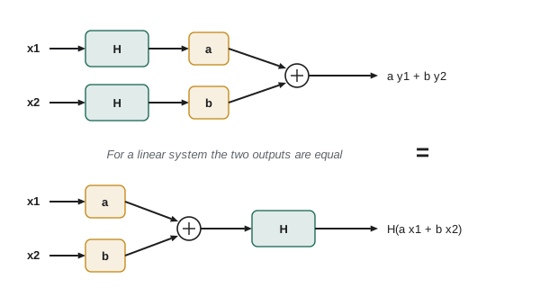
Linearity
A system is linear if it obeys the superposition principle. For any inputs \( x_1 \) and \( x_2 \) with outputs \( y_1 \) and \( y_2 \), and any constants a and b:
Superposition combines two properties: homogeneity (doubling the input doubles the output) and additivity (the response to a sum is the sum of the responses). It is enormously useful. It means we can break a complicated input into simple pieces, such as steps, impulses or sinusoids, find the response to each piece, and add the results. Lesson 1 already used this to build a ramp-and-hold command from two ramps; lesson 3 will build every input from impulses, and lesson 8 from sinusoids.
A quick test catches many nonlinear systems: a linear system must give zero output for zero input. A sensor with a constant offset, \( y = 2x + 0.5 \), therefore fails the strict test, even though its graph is a straight line; engineers call such a system affine, and handle it by subtracting the offset and working with deviations. Common nonlinearities in robots include saturation (a motor driver cannot exceed its supply voltage, a joint cannot exceed its range), dead zones (static friction means small torques produce no motion), backlash in gears (ROB-220), quantization in encoders and ADCs, products of variables such as the Coriolis terms in manipulator dynamics, and trigonometric functions such as the gravity torque \( mgl\sin\theta \) on a link.
Worked problem
Testing for linearity
Which of these systems are linear? (a) \( y(t) = 3\,\dot{x}(t) \); (b) \( y(t) = x(t)^2 \); (c) \( y(t) = t\,x(t) \); (d) a motor driver \( y = \text{sat}(x) \) that clips at ±24 V.
Show solution
- (a) Differentiation is linear: \( 3\frac{d}{dt}(ax_1 + bx_2) = a(3\dot{x}_1) + b(3\dot{x}_2) \). Linear.
- (b) \( (ax_1)^2 = a^2x_1^2 \neq a\,x_1^2 \). Fails homogeneity. Nonlinear.
- (c) \( t(ax_1 + bx_2) = a\,t\,x_1 + b\,t\,x_2 \). Linear, although, as the next section shows, not time-invariant.
- (d) An input of 20 V gives 20 V, but 40 V gives 24 V, not 40 V. Nonlinear once saturation is reached.
Answer: Systems (a) and (c) are linear; (b) and (d) are not. The driver is linear only while commands stay within ±24 V, which is why controllers include anti-windup logic for when they saturate (ROB-300).
Time invariance
A system is time-invariant if its behaviour does not change with time: delaying the input simply delays the output by the same amount. Formally, if \( x(t) \) produces \( y(t) \), then \( x(t - t_0) \) produces \( y(t - t_0) \) for every shift \( t_0 \). A gearbox is time-invariant; so is a filter with fixed coefficients. A system whose parameters drift is time-varying: a battery-powered drive whose maximum torque falls as the battery discharges, a drone whose mass decreases as it drops payload, or a robot arm whose effective inertia at the shoulder depends on the configuration of the elbow (ROB-300). The system \( y = t\,x(t) \) from the example above is time-varying, because the multiplier t means the same input applied later is amplified more.
In practice, most parameters change slowly compared with the dynamics of interest, so a time-invariant model, perhaps updated occasionally, works well. The arm's inertia changes as it moves, but over the few milliseconds of a current-loop transient it is effectively constant. Adaptive controllers and gain scheduling exist for the cases where this approximation breaks down.
Worked problem
Checking time invariance
Is the averaging system \( y(t) = \frac{1}{2}\int_{t-2}^{t} x(\tau)\,d\tau \) time-invariant? Is \( y(t) = x(2t) \)?
Show solution
- For the average, shift the input: \( x_2(t) = x(t - t_0) \). Then \( y_2(t) = \tfrac{1}{2}\int_{t-2}^{t} x(\tau - t_0)\,d\tau \). Substituting \( \sigma = \tau - t_0 \) gives \( \tfrac{1}{2}\int_{t-t_0-2}^{t-t_0} x(\sigma)\,d\sigma = y(t - t_0) \). Time-invariant.
- For \( y(t) = x(2t) \): the shifted input gives \( y_2(t) = x(2t - t_0) \), but the shifted output is \( y(t - t_0) = x(2t - 2t_0) \). These differ. Time-varying.
Answer: The two-second moving average is time-invariant; the time compressor is not. A recorded trajectory played back at double speed is the second kind of operation, which is why its effect cannot be described by a fixed filter.
Causality and memory
A system is causal if its output at any time depends only on present and past inputs, never future ones. Every physical system is causal: a motor cannot respond to a voltage before it is applied. Causality matters in software, because it is tempting to write filters that use future samples. A centred moving average, \( y[n] = (x[n-1] + x[n] + x[n+1])/3 \), is non-causal and cannot run in real time; it can only be applied after the fact, to logged data. Offline processing, such as smoothing a recorded trajectory or analysing a test, may legitimately use non-causal filters, and the zero-phase filtering of lesson 11 does exactly that.
A system is memoryless, or static, if its output depends only on the present input: an ideal gearbox \( \theta_{\text{out}} = \theta_{\text{in}}/N \) or a potentiometer. Systems with memory are dynamic: their output depends on the history of the input, because they store energy or information. A motor stores kinetic energy in its rotor and magnetic energy in its windings; an integrator accumulates its input; a digital filter stores past samples. Dynamic systems are described by differential or difference equations, and their study occupies most of this course.
Stability
Stability is the most important property of all, because an unstable robot can damage itself and hurt people. The most common definition for signals and systems is bounded-input, bounded-output (BIBO) stability: every bounded input produces a bounded output. An integrator is not BIBO-stable, because a constant input, which is bounded, produces a ramp that grows without limit. An inverted pendulum balancing robot without control is unstable: the smallest disturbance grows exponentially. A properly tuned feedback loop can make an unstable plant stable, and a poorly tuned one can make a stable plant unstable; lesson 6 shows how.
For LTI systems, stability can be read directly from the system's description. Lesson 3 shows that a continuous LTI system is BIBO-stable exactly when its impulse response is absolutely integrable; lesson 5 translates this into the condition that all poles of the transfer function lie in the left half of the complex plane; and lesson 10 gives the discrete-time equivalent, poles inside the unit circle. These tests are what make LTI theory so practical: stability can be checked by computation rather than by waiting to see whether the robot shakes itself apart.
Worked problem
Spotting instability
Classify each system as BIBO-stable or not: (a) \( y(t) = \int_{-\infty}^{t} x(\tau)\,d\tau \); (b) \( \dot{y} = -2y + x \); (c) \( \dot{y} = 3y + x \); (d) \( y[n] = 0.9\,y[n-1] + x[n] \).
Show solution
- (a) A unit step input gives a ramp output. Unbounded, so unstable.
- (b) The natural response is \( e^{-2t} \), which decays; a bounded input gives a bounded output. Stable.
- (c) The natural response is \( e^{3t} \), which grows. Unstable.
- (d) The natural response is \( 0.9^n \), which decays. A constant input of 1 settles at \( 1/(1 - 0.9) = 10 \). Stable.
Answer: Systems (b) and (d) are stable; (a) and (c) are not. The sign of the coefficient on y, or the size of the coefficient in the difference equation, decides the matter, a pattern lessons 5 and 10 formalize with poles.
LTI systems and why they matter
Systems that are both linear and time-invariant have a remarkable property: they are completely characterized by a single function, the impulse response, and the output for any input can be computed from it by convolution (lesson 3). Equivalently, they are characterized by their transfer function (lesson 5) or frequency response (lesson 7). Complex exponentials pass through them unchanged in shape, only scaled and shifted, so sinusoidal inputs produce sinusoidal outputs at the same frequency. None of this holds for nonlinear or time-varying systems, for which analysis is much harder and often only simulation will do.
| Property | Meaning | Robot example that has it | Robot example that lacks it |
|---|---|---|---|
| Linear | Superposition holds | Small-motion motor model | Saturated driver; gravity torque at large angles |
| Time-invariant | Behaviour does not change with time | Fixed-gain filter | Drone losing mass; draining battery |
| Causal | Output depends only on past and present input | Every physical system | Centred moving average on logged data |
| Memoryless | Output depends only on present input | Ideal gearbox; potentiometer | Motor with rotor inertia |
| BIBO-stable | Bounded input gives bounded output | Damped joint under PID | Uncontrolled balancing robot |
Linearization: using LTI tools on nonlinear robots
Because real robots are nonlinear, how can LTI theory apply? The answer is linearization. Near an operating point, any smooth nonlinear function looks like a straight line, its tangent. If the robot stays close to the operating point, small deviations from it obey a linear model. For a function f of one variable near \( x_0 \), the first-order Taylor approximation is
For a pendulum hanging straight down, the gravity torque \( -mgl\sin\theta \) becomes \( -mgl\,\theta \) for small angles, because \( \sin\theta \approx \theta \); the error is under 1 % for angles up to about 14°. For an inverted pendulum balancing upright, the same procedure gives a torque of \( +mgl\,\delta\theta \), whose positive sign signals instability. Linearized models underlie nearly all classical robot control design: the controller is designed for the linear model and then tested, in simulation and on hardware, on the real nonlinear robot.
Worked problem
Linearizing a link under gravity
A 0.5 kg link has its centre of mass 0.3 m from the joint. Gravity torque is \( \tau_g = mgl\cos\theta \), with θ measured from the horizontal. Linearize about \( \theta_0 = 30° \) and estimate the torque at 32°.
Show solution
- \( \tau_g(\theta_0) = 0.5 \times 9.81 \times 0.3 \times \cos 30° = 1.274 \) N·m.
- Slope: \( d\tau_g/d\theta = -mgl\sin\theta_0 = -1.4715 \times 0.5 = -0.736 \) N·m/rad.
- \( \delta\theta = 2° = 0.0349 \) rad, so \( \tau_g \approx 1.274 - 0.736 \times 0.0349 = 1.249 \) N·m.
- Exact: \( 1.4715\cos 32° = 1.248 \) N·m.
Answer: The linear model predicts 1.249 N·m against an exact 1.248 N·m, an error under 0.1 %. Linearization works well for small deviations; for a 30° swing it would be poor, and the controller would need gain scheduling or gravity compensation.
import numpy as np
m, g, l = 0.5, 9.81, 0.3
th0 = np.radians(30)
for d_deg in [2, 5, 10, 20, 40]:
    d = np.radians(d_deg)
    exact = m*g*l*np.cos(th0 + d)
    lin = m*g*l*np.cos(th0) - m*g*l*np.sin(th0)*d
print(f"deviation {d_deg:2d} deg: exact {exact:6.3f} linear {lin:6.3f} error {100*(lin-exact)/exact:6.2f} %")deviation 2 deg: exact 1.248 linear 1.249 error 0.06 % deviation 5 deg: exact 1.205 linear 1.210 error 0.40 % deviation 10 deg: exact 1.127 linear 1.146 error 1.66 % deviation 20 deg: exact 0.946 linear 1.018 error 7.58 % deviation 40 deg: exact 0.503 linear 0.761 error 51.15 %
The error stays negligible for a few degrees and grows roughly with the square of the deviation, as the neglected second-order Taylor term predicts. This is the practical meaning of small-signal: close enough to the operating point that the curvature does not matter.
Common mistakes
MistakeCalling y = 2x + 3 linear because its graph is a straight line
InsteadIt fails superposition because of the offset; treat it as affine and work with deviations.
MistakeAssuming linearity implies time invariance
InsteadThey are independent: y = t·x(t) is linear but time-varying.
MistakeRunning a centred moving average in a real-time loop
InsteadIt needs future samples; use a causal filter online and keep non-causal smoothing for logged data.
MistakeTreating an integrator as stable because it never oscillates
InsteadA constant input makes its output grow without bound, so it is not BIBO-stable.
MistakeUsing a linearized model far from its operating point
InsteadCheck the size of deviations; the error grows with the neglected higher-order terms.
Summary and key terms
- A system maps input signals to output signals and can be drawn as a block; blocks connect in series, parallel and feedback.
- Linear systems obey superposition: the response to a weighted sum is the weighted sum of the responses.
- Time-invariant systems behave the same whenever the input is applied.
- Causal systems depend only on present and past inputs; every physical system is causal.
- Systems with memory store energy or information and are described by differential or difference equations.
- BIBO stability means every bounded input gives a bounded output; integrators and inverted pendulums are not stable.
- Linearization about an operating point lets LTI tools be applied to nonlinear robots for small deviations.
- System
- A process that transforms an input signal into an output signal.
- Superposition
- The principle that the response to a weighted sum of inputs is the same weighted sum of responses.
- Linear system
- A system that obeys superposition.
- Time-invariant system
- A system whose response to a delayed input is the delayed response.
- LTI system
- A system that is both linear and time-invariant.
- Causal system
- A system whose output does not depend on future inputs.
- Memoryless system
- A system whose output depends only on the present input.
- BIBO stability
- Every bounded input produces a bounded output.
- Operating point
- The steady condition about which a nonlinear system is linearized.
- Linearization
- Approximating a nonlinear system by its first-order Taylor expansion near an operating point.
Practice problems
Work each problem on paper first, then reveal the answer to check.
Is \( y(t) = x(t - 2) \) linear, time-invariant and causal?
Show answer
Yes to all three: it is a pure two-second delay.
Is \( y(t) = x(t + 1) \) causal?
Show answer
No; it needs the input one second in the future.
Is \( y = |x| \) linear?
Show answer
No; with a = −1, \( |-x| = |x| \neq -|x| \).
Is \( y[n] = x[n] - x[n-1] \) stable?
Show answer
Yes; a bounded input gives an output bounded by twice the input bound.
Is \( y[n] = y[n-1] + x[n] \) stable?
Show answer
No; it is a discrete integrator (accumulator), and a constant input gives a ramp.
A motor driver saturates at ±12 V. For what inputs is it linear?
Show answer
For inputs between −12 V and +12 V.
Linearize \( f(x) = x^2 \) about \( x_0 = 3 \).
Show answer
\( f \approx 9 + 6\,\delta x \).
For which angles is \( \sin\theta \approx \theta \) accurate to 1 %?
Show answer
Up to about 14° (0.24 rad).
Give a robot example of a time-varying system.
Show answer
A drone dropping payload, or a drive whose torque limit falls as the battery drains.
Why do LTI systems keep sinusoids sinusoidal?
Show answer
Complex exponentials are eigenfunctions of LTI systems, so only amplitude and phase change.
Lesson quiz · 5 questions
Score 60% or more to complete this lesson.
Create a free account to save your progress, take quizzes and earn a certificate.