
ROB-230 · Lesson 5 of 12 · 31 min
The Laplace transform and transfer functions
Solving differential equations directly and evaluating convolution integrals by hand both become laborious as soon as systems grow beyond second order or are connected together. The Laplace transform removes most of that labour. It converts linear differential equations with constant coefficients into algebraic equations in a complex variable s, and it converts convolution into simple multiplication. The ratio of output to input transforms, the transfer function, becomes a compact description of an LTI system, and the roots of its denominator, the poles, reveal stability and the shape of the response at a glance. Transfer functions are the native language of classical control: motor models, sensor models, filters and controllers are all written as ratios of polynomials in s, and the block diagrams of lesson 6 multiply them together. This lesson builds the transform, the key pairs and properties, partial-fraction inversion, poles and zeros, and the final value theorem.
The transform
For a causal signal f(t), zero for t < 0, the (one-sided) Laplace transform is
The transform weighs the signal against decaying complex exponentials \( e^{-st} \) and records how much of each is present. For many signals the integral converges only when the real part of s exceeds some value, which defines the region of convergence; for the causal signals used in engineering we rarely need to worry about it, as long as we remember that the transform describes behaviour for t ≥ 0. Starting the integral at \( 0^- \), just before zero, makes sure that an impulse at t = 0 is included.
Worked problem
Transforming an exponential
Find the Laplace transform of \( f(t) = e^{-at}u(t) \).
Show solution
- \( F(s) = \int_0^{\infty} e^{-at}e^{-st}\,dt = \int_0^{\infty} e^{-(s+a)t}\,dt \).
- \( = \left[-\frac{e^{-(s+a)t}}{s+a}\right]_0^{\infty} = \frac{1}{s+a} \), provided Re(s) > −a so the upper limit vanishes.
Answer: \( \mathcal{L}\{e^{-at}u(t)\} = 1/(s + a) \). Setting a = 0 gives the transform of the unit step, 1/s. Almost every other pair can be built from this one.
Key transform pairs and properties
In practice nobody evaluates the integral every time. A short table of pairs and a few properties cover nearly every problem met in robotics.
| Signal f(t), t ≥ 0 | Transform F(s) |
|---|---|
| Unit impulse \( \delta(t) \) | 1 |
| Unit step \( u(t) \) | \( 1/s \) |
| Ramp \( t \) | \( 1/s^2 \) |
| Exponential \( e^{-at} \) | \( 1/(s + a) \) |
| \( t\,e^{-at} \) | \( 1/(s + a)^2 \) |
| Sine \( \sin\omega t \) | \( \omega/(s^2 + \omega^2) \) |
| Cosine \( \cos\omega t \) | \( s/(s^2 + \omega^2) \) |
| Damped sine \( e^{-at}\sin\omega t \) | \( \omega/((s + a)^2 + \omega^2) \) |
| Damped cosine \( e^{-at}\cos\omega t \) | \( (s + a)/((s + a)^2 + \omega^2) \) |
The properties are what make the transform powerful:
- Linearity: \( \mathcal{L}\{af + bg\} = aF + bG \).
- Differentiation: \( \mathcal{L}\{\dot{f}\} = sF(s) - f(0^-) \), and \( \mathcal{L}\{\ddot{f}\} = s^2F(s) - sf(0^-) - \dot{f}(0^-) \). Differentiation becomes multiplication by s, with initial conditions appearing as extra terms.
- Integration: \( \mathcal{L}\{\int_0^t f\,d\tau\} = F(s)/s \). Integration becomes division by s, which is why 1/s is the symbol of an integrator in block diagrams.
- Time delay: \( \mathcal{L}\{f(t - T)u(t - T)\} = e^{-sT}F(s) \). A transport delay, such as communication latency, multiplies by \( e^{-sT} \).
- Convolution: \( \mathcal{L}\{f * g\} = F(s)\,G(s) \). The integral of lesson 3 becomes a product.
- Final value theorem: if all poles of sF(s) are in the left half-plane, \( \lim_{t\to\infty} f(t) = \lim_{s\to 0} sF(s) \).
Transfer functions
Take the Laplace transform of an LTI differential equation with all initial conditions zero. For the standard first-order system \( \tau\dot{y} + y = Kx \), the differentiation property gives \( \tau sY(s) + Y(s) = KX(s) \), so
The transfer function G(s) is the ratio of the output transform to the input transform. Because \( Y(s) = G(s)X(s) \) and the output is the input convolved with the impulse response, G(s) is simply the Laplace transform of the impulse response. For the second-order system of lesson 4,
and for a DC motor with the inductance kept, eliminating the current from the electrical and mechanical equations gives the transfer function from voltage to speed:
Position is the integral of speed, so the voltage-to-angle transfer function has an extra factor 1/s. Writing transfer functions takes practice but follows one rule: transform each equation, replace each derivative by s, and solve algebraically for the output over the input.
Worked problem
Transfer function of a mass-spring-damper
A camera on a flexible mount has m = 0.5 kg, b = 4 N·s/m and k = 200 N/m. Find the transfer function from applied force to displacement, and its \( \omega_n \) and \( \zeta \).
Show solution
- Transform \( m\ddot{x} + b\dot{x} + kx = F \) with zero initial conditions: \( (ms^2 + bs + k)X = F \).
- \( G(s) = \dfrac{1}{0.5s^2 + 4s + 200} = \dfrac{2}{s^2 + 8s + 400} \).
- Compare with the standard form: \( \omega_n^2 = 400 \), so \( \omega_n = 20 \) rad/s; \( 2\zeta\omega_n = 8 \), so \( \zeta = 0.2 \).
- Steady-state gain \( G(0) = 2/400 = 0.005 \) m/N.
Answer: \( G(s) = 2/(s^2 + 8s + 400) \), with \( \omega_n \) = 20 rad/s (3.2 Hz) and ζ = 0.2, a lightly damped mount that will ring with about 53 % overshoot when bumped. A 1 N steady push deflects it 5 mm.
Poles and zeros
A rational transfer function is a ratio of polynomials, which can be factored:
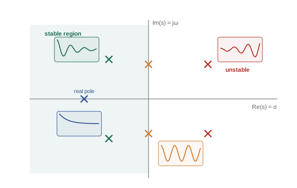
The roots \( z_i \) of the numerator are the zeros; the roots \( p_i \) of the denominator are the poles, which are exactly the roots of the characteristic equation of lesson 4. Each real pole at \( s = -a \) contributes a term \( e^{-at} \) to the impulse response; each complex pair \( -\sigma \pm j\omega_d \) contributes a decaying oscillation \( e^{-\sigma t}\sin(\omega_d t + \phi) \). The pole locations therefore tell the whole story of the natural response:
- Poles in the left half-plane (negative real part) give decaying terms. If all poles are there, the system is stable.
- Any pole in the right half-plane gives a growing term: instability.
- Poles on the imaginary axis give sustained oscillation (a pair) or a constant or ramp (at the origin); such systems, including integrators, are called marginally stable and are not BIBO-stable.
- Distance from the imaginary axis sets decay rate; distance from the real axis sets oscillation frequency. Poles far to the left die out fast; the poles nearest the imaginary axis, called dominant poles, dominate the response.
Zeros do not affect stability but shape the response: a zero near a pole partly cancels it, and a zero in the right half-plane, which appears for example in some flexible-link arms and in the tilt dynamics of balancing robots, makes the response initially move the wrong way, which limits how fast such a system can be controlled.
Inverting transforms by partial fractions
To get a time response from a transform, factor the denominator and split the rational function into simple terms whose inverses are in the table. For distinct real poles,
This cover-up rule finds each coefficient by cancelling its factor and substituting the pole. Repeated poles and complex pairs need slightly more work, but the idea is the same.
Worked problem
Step response by partial fractions
A joint's closed-loop transfer function is \( G(s) = 6/((s + 2)(s + 3)) \). Find its unit step response.
Show solution
- \( Y(s) = G(s)\cdot\frac{1}{s} = \frac{6}{s(s + 2)(s + 3)} \).
- Cover-up: \( A_0 = 6/(2 \times 3) = 1 \); \( A_1 = 6/((-2)(1)) = -3 \) at s = −2; \( A_2 = 6/((-3)(-1)) = 2 \) at s = −3.
- \( Y(s) = \frac{1}{s} - \frac{3}{s + 2} + \frac{2}{s + 3} \).
- Invert term by term: \( y(t) = 1 - 3e^{-2t} + 2e^{-3t} \) for t ≥ 0.
Answer: \( y(t) = 1 - 3e^{-2t} + 2e^{-3t} \). Check: y(0) = 1 − 3 + 2 = 0 and y(∞) = 1, as expected for a system with unit gain starting from rest. The slower pole at −2 dominates the later part of the response.
The final and initial value theorems
Often we need only the steady state: where will the joint end up, what steady error remains? The final value theorem answers without inverting anything. For the joint above, \( \lim_{s\to 0} s \cdot \frac{6}{s(s+2)(s+3)} = 1 \). The theorem applies only if the response actually settles, meaning all poles of sY(s) are in the left half-plane; applying it to an unstable system gives a meaningless number. A companion initial value theorem, \( f(0^+) = \lim_{s\to\infty} sF(s) \), gives the starting value.
Worked problem
Steady-state error with a disturbance
A motor speed loop has closed-loop transfer function from a load-torque disturbance D to speed error E of \( E(s)/D(s) = 0.5/(s + 10) \). A constant 2 N·m disturbance is applied. What steady speed error results? What if an integrator in the controller changes the transfer function to \( 0.5s/(s^2 + 10s + 40) \)?
Show solution
- Constant disturbance: D(s) = 2/s.
- Without integral action: \( e_{ss} = \lim_{s\to 0} s \cdot \frac{0.5}{s + 10}\cdot\frac{2}{s} = 1/10 = 0.1 \) rad/s.
- With integral action: \( e_{ss} = \lim_{s\to 0} s \cdot \frac{0.5s}{s^2 + 10s + 40}\cdot\frac{2}{s} = 0 \). The poles of \( s^2 + 10s + 40 \) have real part −5, so the theorem applies.
Answer: A steady error of 0.1 rad/s without integral action, and zero with it. The zero at s = 0 introduced by the integrator is exactly what removes constant disturbances, which is why almost every robot joint controller includes integral action (ROB-300).
Working with transfer functions in software
Transfer functions are stored as coefficient lists, highest power first. NumPy can find poles and zeros with np.roots, and the step response can be computed by partial fractions or by simulation. The code below finds the poles of the camera-mount model and checks the partial-fraction step response of the joint example against a direct numerical simulation.
import numpy as np
den = [1, 8, 400]                       # camera mount: 2/(s^2 + 8s + 400)
p = np.roots(den)
wn = np.sqrt(den[2]); zeta = den[1]/(2*wn)
print("poles:", np.round(p, 3), " wn =", wn, " zeta =", zeta)
# joint: G = 6/((s+2)(s+3)); compare partial fractions with simulation
h, T = 1e-4, 4.0
x1 = x2 = 0.0                            # y'' + 5y' + 6y = 6u
for k in range(int(T/h)):
    a = 6.0 - 5.0*x2 - 6.0*x1
    x1, x2 = x1 + h*x2, x2 + h*a
t = T
pf = 1 - 3*np.exp(-2*t) + 2*np.exp(-3*t)
print(f"y(4 s): simulation {x1:.5f}, partial fractions {pf:.5f}")poles: [-4.+19.596j -4.-19.596j] wn = 20.0 zeta = 0.2 y(4 s): simulation 0.99901, partial fractions 0.99901
The poles at −4 ± 19.6j confirm ζ = 0.2 and a damped ringing frequency of 19.6 rad/s, and the simulated and analytical step responses agree to five decimal places, confirming the partial-fraction result.
Common mistakes
MistakeKeeping initial conditions when deriving a transfer function
InsteadTransfer functions assume zero initial conditions; handle nonzero ones separately.
MistakeApplying the final value theorem to an unstable system
InsteadCheck that all poles of sF(s) are in the left half-plane first.
MistakeForgetting the factor 1/s for a step input
InsteadThe output transform is G(s) times 1/s for a unit step.
MistakeThinking zeros determine stability
InsteadStability depends only on the poles; zeros shape the response.
MistakeTreating a pole at the origin as stable because nothing grows exponentially
InsteadAn integrator is marginally stable and not BIBO-stable.
Summary and key terms
- The Laplace transform turns linear differential equations into algebraic equations in s.
- Differentiation becomes multiplication by s, integration division by s, and a delay multiplication by \( e^{-sT} \).
- Convolution in time becomes multiplication of transforms.
- A transfer function is the ratio of output to input transforms with zero initial conditions, and equals the transform of the impulse response.
- Poles are roots of the denominator; their locations set stability, decay rates and oscillation frequencies.
- Partial fractions invert rational transforms into sums of exponentials and damped sinusoids.
- The final value theorem gives the steady state of a stable system without inverting the transform.
- Laplace transform
- The integral \( \int_0^\infty f(t)e^{-st}dt \) that maps a signal to a function of complex s.
- Complex frequency
- The variable \( s = \sigma + j\omega \).
- Transfer function
- The ratio Y(s)/X(s) of an LTI system with zero initial conditions.
- Pole
- A root of the transfer function denominator.
- Zero
- A root of the transfer function numerator.
- Dominant poles
- The poles closest to the imaginary axis, which dominate the response.
- Partial fractions
- Splitting a rational function into simple terms for inversion.
- Final value theorem
- The rule \( f(\infty) = \lim_{s\to 0} sF(s) \) for a settling response.
- Marginally stable
- Having poles on the imaginary axis but none in the right half-plane.
- Right-half-plane zero
- A zero with positive real part that causes an initial wrong-way response.
Practice problems
Work each problem on paper first, then reveal the answer to check.
Find the Laplace transform of \( 3 + 2e^{-4t} \).
Show answer
\( 3/s + 2/(s + 4) \).
Write the transfer function of \( 2\dot{y} + 8y = 4x \).
Show answer
\( 4/(2s + 8) = 2/(s + 4) \).
What are the poles of \( 1/(s^2 + 6s + 25) \)?
Show answer
\( -3 \pm 4j \).
Is \( G(s) = 1/(s^2 - s + 4) \) stable?
Show answer
No; its poles have real part +0.5.
Find the steady-state response of \( 10/(s + 5) \) to a unit step.
Show answer
2.
Invert \( 1/(s(s + 1)) \).
Show answer
\( 1 - e^{-t} \).
What transfer function represents a 50 ms communication delay?
Show answer
\( e^{-0.05s} \).
A motor speed model is \( 20/(0.08s + 1) \). What is the transfer function from voltage to angle?
Show answer
\( 20/(s(0.08s + 1)) \).
Find \( \omega_n \) and ζ for \( 9/(s^2 + 3s + 9) \).
Show answer
\( \omega_n = 3 \) rad/s, ζ = 0.5.
Use the initial value theorem on \( F(s) = (2s + 1)/(s + 3) \) times 1/s. What is f(0+)?
Show answer
\( \lim_{s\to\infty} (2s + 1)/(s + 3) = 2 \).
Lesson quiz · 5 questions
Score 60% or more to complete this lesson.
Create a free account to save your progress, take quizzes and earn a certificate.