
ROB-230 · Lesson 6 of 12 · 31 min
Block diagrams and feedback
A robot joint is not a single transfer function but a chain of them: a controller drives a power amplifier, which drives a motor, which turns a gearbox and a link, whose angle is measured by an encoder and compared with the command. Block diagrams make such chains visible, and the algebra of transfer functions lets us collapse them into a single input-output relation. The most important structure in any block diagram is the feedback loop, in which the output is measured and used to correct the input. Feedback is the reason robots can hold position against gravity, track trajectories despite friction and keep working when parameters change, and it is also the reason they can oscillate or go unstable when tuned badly. This lesson develops block-diagram algebra, derives the closed-loop transfer function, and explains what feedback buys: disturbance rejection, reduced sensitivity to parameter changes, and the ability to move poles. Designing the controller itself is the subject of ROB-300; here the aim is to understand what a loop does to the signals passing through it.
Block diagram elements and algebra
A block diagram has three elements: blocks, each containing a transfer function that multiplies its input; summing junctions, which add or subtract signals according to the signs marked on them; and pickoff points, where a signal is copied to two destinations without being changed. Three rules reduce most diagrams.
- Series: blocks \( G_1 \) and \( G_2 \) in cascade combine into \( G_1G_2 \). This follows from the convolution property of lesson 5 and requires that the second block does not load the first, which holds for signals in software and for buffered electronics but needs care with mechanical and electrical connections.
- Parallel: blocks sharing an input with outputs added combine into \( G_1 + G_2 \).
- Feedback: a forward block G with a feedback block H subtracted at the input combines into \( G/(1 + GH) \), derived below.
Pickoff points and summing junctions can also be moved past blocks, provided compensating blocks are inserted, which helps when untangling complicated diagrams. With these rules any diagram built from linear blocks reduces to a single transfer function, although for large systems the state-space methods of lesson 12 are more systematic.
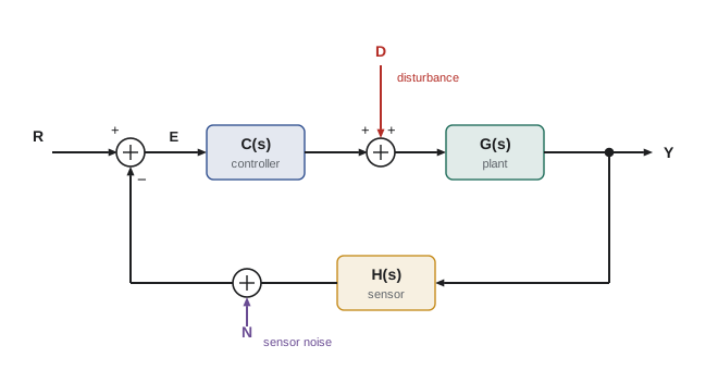
The closed-loop transfer function
Consider the standard loop: a reference R, an error \( E = R - HY \), a controller C and plant G in the forward path, so \( Y = CGE \), and a sensor H in the feedback path. Substituting the error,
The product \( L(s) = C(s)G(s)H(s) \), the gain around the loop, is called the loop transfer function or open-loop transfer function. It is the single most important quantity in feedback design. The denominator \( 1 + L(s) \) sets the closed-loop poles: they are the roots of \( 1 + L(s) = 0 \), the closed-loop characteristic equation. Feedback therefore moves poles. A plant with poles in an awkward place, or even in the right half-plane, can be given well-damped closed-loop poles by choosing C. When the loop gain is large, \( Y/R \approx 1/H \): the output follows the reference scaled by the sensor, almost regardless of the plant. This is the essential magic of feedback, and also its main requirement: the sensor must be accurate, because the loop faithfully tracks whatever the sensor reports.
Worked problem
Closing a loop around a motor
A motor's speed responds to voltage as \( G(s) = 20/(0.08s + 1) \) rad/s per volt. A proportional controller \( C = K_p \) (volts per rad/s of error) and an ideal tachometer (H = 1) close the loop. Find the closed-loop transfer function, time constant and steady-state gain for \( K_p = 0.2 \).
Show solution
- \( \frac{Y}{R} = \frac{K_pG}{1 + K_pG} = \frac{20K_p}{0.08s + 1 + 20K_p} \).
- With \( K_p = 0.2 \): \( \frac{4}{0.08s + 5} = \frac{0.8}{0.016s + 1} \).
- Closed-loop time constant 0.016 s, five times faster than the open-loop 0.08 s.
- Steady-state gain 0.8: a command of 100 rad/s settles at 80 rad/s.
Answer: Feedback made the motor five times faster, moving its pole from −12.5 to −62.5 rad/s, but proportional control alone leaves a 20 % steady error. Raising \( K_p \) reduces the error and speeds the response further, until saturation, noise or neglected dynamics intervene; adding integral action removes the steady error entirely, as lesson 5 showed.
Steady-state error and system type
How well a loop tracks a reference in steady state depends on how many integrators, poles at s = 0, the loop transfer function contains. With unity feedback the error is \( E = R/(1 + L) \), and the final value theorem gives the steady error for standard inputs:
| Loop type (integrators in L) | Step input error | Ramp input error | Example |
|---|---|---|---|
| Type 0 (none) | \( 1/(1 + K_p) \), with \( K_p = L(0) \) | Infinite | Proportional speed control of a motor |
| Type 1 (one) | Zero | \( 1/K_v \), with \( K_v = \lim sL(s) \) | Proportional position control (the motor integrates speed to angle) |
| Type 2 (two) | Zero | Zero | PI position control tracking a constant-velocity conveyor |
This explains a classic observation. A position loop on a motor naturally contains one integrator, because angle is the integral of speed, so proportional position control reaches a step target exactly (in the absence of friction and gravity) but lags a ramp, such as a moving conveyor, by a constant amount. Adding integral action raises the type and removes that lag.
Worked problem
Tracking a conveyor
A pick-and-place axis has loop transfer function \( L(s) = 50/(s(0.05s + 1)) \). It must track a conveyor moving at 0.3 m/s. What is the steady following error?
Show solution
- The loop is type 1. Velocity constant \( K_v = \lim_{s\to 0} sL(s) = 50 \) s⁻¹.
- Ramp of slope 0.3 m/s gives error \( 0.3/K_v = 0.3/50 = 0.006 \) m.
Answer: A constant lag of 6 mm behind the conveyor. If the gripper needs 2 mm accuracy, either \( K_v \) must triple, which may make the loop oscillate, or a velocity feedforward term or integral action must be added to remove the lag.
Disturbance rejection
Robots are constantly pushed by disturbances: gravity on a link, friction in a gearbox, a payload picked up, wind on a drone. In the standard loop, a disturbance D added at the plant input reaches the output through
Compared with the open-loop effect G, feedback divides the disturbance by \( 1 + L \). Wherever the loop gain is large, typically at low frequencies, disturbances are strongly suppressed. A joint holding position against a slowly varying load hardly moves; a sudden fast push still gets through, because no practical loop has high gain at high frequency. The frequency-domain view of lesson 7 makes this precise: disturbance rejection is good below the loop's bandwidth and absent above it.
Worked problem
Rejecting a load disturbance
For the motor loop above with \( K_p = 0.2 \), a load torque appears as an equivalent disturbance voltage of 1 V at the plant input. How much does the steady speed change, with and without feedback?
Show solution
- Open loop: \( \Delta\omega = G(0) \times 1 = 20 \) rad/s.
- Closed loop: \( G(0)/(1 + K_pG(0)) = 20/(1 + 4) = 4 \) rad/s.
Answer: Feedback cuts the speed drop from 20 rad/s to 4 rad/s, a factor of \( 1 + L(0) = 5 \). A larger gain, or integral action, would reduce it further, the latter to zero.
Sensitivity to parameter changes and to noise
Plants change: batteries sag, loads vary, friction rises in the cold. The sensitivity of the closed-loop transfer function T to changes in the plant G is
so a 10 % change in the plant produces only a \( 10/(1 + L) \) % change in closed-loop behaviour. With L = 9, a 10 % plant change becomes a 1 % change in the loop. This robustness is the original reason feedback amplifiers were invented in 1927, and it is why a well-tuned robot joint behaves consistently even though its motor and gearbox vary from unit to unit. The function \( S = 1/(1 + L) \) is called the sensitivity function, and its partner \( T = L/(1 + L) \) the complementary sensitivity; note that \( S + T = 1 \).
Feedback has a price. Sensor noise N enters the loop at the same point as the reference, so the output responds to noise through T, just as it responds to commands. A loop with high gain at high frequency faithfully reproduces the noise of its sensor, making motors hum and links chatter. Because S + T = 1, we cannot make both small at the same frequency: we want S small at low frequencies for tracking and disturbance rejection, and T small at high frequencies to ignore noise. Managing this trade-off is the core of loop shaping in ROB-300, and it is one reason sensor filtering (lesson 11) must be designed together with the controller.
Worked problem
Robustness to a battery sag
For the motor loop with \( K_p = 0.2 \), the battery sags and the plant gain falls from 20 to 16 rad/s per volt (−20 %). How much does the closed-loop steady gain change?
Show solution
- Before: \( T(0) = 4/(1 + 4) = 0.800 \).
- After: \( L(0) = 0.2 \times 16 = 3.2 \), \( T(0) = 3.2/4.2 = 0.762 \).
- Change: \( (0.762 - 0.800)/0.800 = -4.8 \) %, close to \( -20 \% \times S = -20/5 = -4 \) % predicted by the sensitivity formula (the small difference is because the change is not infinitesimal).
Answer: The 20 % plant change becomes a change of about 5 % in closed-loop behaviour. With integral action the steady gain would stay at exactly 1 regardless.
Feedback, delay and instability
Feedback can also destabilize. If the loop gain is high and the signal coming back around the loop is delayed or phase-shifted enough, the correction arrives late and pushes in the wrong direction, reinforcing the error instead of reducing it. Every real loop contains such delays: sample-and-hold in the controller (lesson 9), sensor filtering, communication latency, motor inductance and structural flexibility. Lesson 7 shows how to measure the margin of safety in terms of gain and phase. A simple experiment makes the danger concrete: the code below closes a proportional loop around a pure integrator with a small delay, and increases the gain until the response begins to oscillate and then grows.
import numpy as np
h, T, delay = 1e-3, 3.0, 0.05          # 50 ms loop delay
nd = int(delay/h)
for K in [5, 15, 30, 40]:
    y = 0.0
    u_hist = [0.0]*nd                   # buffer of delayed commands
    out = []
    for k in range(int(T/h)):
        u = K*(1.0 - y)                 # proportional control, unit step command
        u_hist.append(u)
        y += h*u_hist.pop(0)            # plant: integrator driven by delayed command
        out.append(y)
    out = np.array(out)
    tail = out[int(2/h):]
print(f"K = {K:2d}: peak {out.max():6.2f}, late swing {tail.max()-tail.min():8.3f}")K = 5: peak 1.00, late swing 0.000 K = 15: peak 1.26, late swing 0.000 K = 30: peak 2.02, late swing 0.740 K = 40: peak 37534.78, late swing 64323.848
At K = 5 the loop settles smoothly; at K = 15 it overshoots by about a quarter; at K = 30, just below the critical value, it is still swinging two seconds later; and at K = 40 the oscillation has grown enormously. Beyond about K = 31, where the loop's phase lag from the 50 ms delay reaches 180° at the frequency where the loop gain is one, the oscillation grows without bound. The critical gain predicted by frequency-response analysis is \( K = \pi/(2 \times 0.05) \approx 31 \) s⁻¹, which lesson 7 explains.
Common mistakes
MistakeWriting the closed loop as G/(1 − GH) for negative feedback
InsteadWith the feedback subtracted at the summing junction, the denominator is 1 + GH.
MistakeAssuming higher gain always improves a loop
InsteadHigher gain improves tracking and rejection but amplifies noise and, with delay, can destabilize.
MistakeTrusting feedback to correct a biased sensor
InsteadThe loop tracks the sensor reading, so a sensor bias becomes an output error.
MistakeExpecting proportional control to remove steady error in a type-0 loop
InsteadA type-0 loop always leaves error 1/(1 + Kp) to a step; add integral action.
MistakeMultiplying blocks that load each other
InsteadSeries multiplication assumes no loading; model coupled physical elements together.
Summary and key terms
- Block diagrams use blocks, summing junctions and pickoff points; series blocks multiply and parallel blocks add.
- The closed-loop transfer function of a negative-feedback loop is CG/(1 + CGH).
- The loop transfer function L = CGH determines the closed-loop poles through 1 + L = 0.
- The number of integrators in the loop sets its type and its steady-state error to steps and ramps.
- Feedback divides disturbances and plant-parameter sensitivity by 1 + L.
- Sensitivity S and complementary sensitivity T satisfy S + T = 1, so tracking and noise rejection trade off.
- Delay and phase lag in a high-gain loop can cause oscillation and instability.
- Block diagram
- A drawing of a system as blocks connected by signals.
- Summing junction
- A point where signals are added or subtracted.
- Pickoff point
- A point where a signal is copied to several destinations.
- Loop transfer function
- The product of all transfer functions around a feedback loop.
- Closed-loop transfer function
- The transfer function from reference to output with the loop closed.
- System type
- The number of pure integrators in the loop transfer function.
- Velocity constant
- The limit of sL(s) as s goes to zero for a type-1 loop.
- Sensitivity function
- \( S = 1/(1 + L) \), which governs disturbance and parameter sensitivity.
- Complementary sensitivity
- \( T = L/(1 + L) \), which governs tracking and noise transmission.
- Disturbance rejection
- The ability of a loop to suppress the effect of external disturbances.
Practice problems
Work each problem on paper first, then reveal the answer to check.
Combine \( G_1 = 2/(s + 1) \) and \( G_2 = 3/s \) in series.
Show answer
\( 6/(s(s + 1)) \).
Find the closed loop for G = 10/(s + 2) with unity feedback.
Show answer
\( 10/(s + 12) \).
A type-0 loop has L(0) = 19. What is its steady error to a unit step?
Show answer
1/20 = 5 %.
A type-1 loop has \( K_v = 100 \) s⁻¹. What is its error tracking a ramp of 2 units/s?
Show answer
0.02 units.
If L(0) = 49, by what factor does feedback reduce a constant disturbance?
Show answer
By 50.
A plant gain drops 30 % in a loop with L = 14. Roughly how much does closed-loop gain change?
Show answer
About 2 %.
What is S + T for any loop?
Show answer
1.
Find the closed-loop poles of L = K/(s(s + 4)) with K = 4.
Show answer
s² + 4s + 4 = 0: a double pole at −2.
Why does a position loop on a motor contain a natural integrator?
Show answer
Angle is the integral of speed.
Name three sources of delay in a digital robot control loop.
Show answer
Sample-and-hold, sensor filtering and communication latency (also computation time).
Lesson quiz · 5 questions
Score 60% or more to complete this lesson.
Create a free account to save your progress, take quizzes and earn a certificate.