Measurement, commutators and the generalized uncertainty principle

Lesson 8 set up the mathematical stage: states are vectors, observables are Hermitian operators. This lesson completes the rules of the game by saying what happens when we measure. The generalized statistical interpretation tells us which results are possible and how likely each is. Commutators of operators tell us which observables can be known together. And from nothing more than the Schwarz inequality we will prove the uncertainty principle in its most general form, a precise statement about the spreads of any two observables, of which Heisenberg's position–momentum relation is one case. The lesson ends with the quantum form of conservation laws: an observable is conserved when its operator commutes with the Hamiltonian.

The generalized statistical interpretation

Suppose the observable \(Q\) has Hermitian operator \(\hat Q\) with a discrete set of orthonormal eigenvectors, \(\hat Q|q_n\rangle = q_n|q_n\rangle\). Because the eigenvectors are complete, any state can be expanded as \(|\psi\rangle = \sum_n c_n|q_n\rangle\) with \(c_n = \langle q_n|\psi\rangle\). The postulate is:

For a continuous spectrum, the probability of a result between \(q\) and \(q + dq\) is \(|\langle q|\psi\rangle|^2dq\). With \(\hat Q = \hat x\) this is Born's original rule, \(|\psi(x)|^2dx\); with \(\hat Q = \hat p\) it is \(|\Phi(p)|^2dp\); with \(\hat Q = \hat H\) it is the rule for energy probabilities used since lesson 3. Normalization guarantees that the probabilities add to one, \(\sum|c_n|^2 = \langle\psi|\psi\rangle = 1\), and the average of the results is the expectation value of lesson 2, \(\sum q_n|c_n|^2 = \langle\psi|\hat Q\psi\rangle\), as inserting the expansion shows.

If the result \(q_n\) belongs to a degenerate eigenvalue, shared by several eigenvectors, the state after measurement is the projection of \(|\psi\rangle\) onto that whole subspace, renormalized. The third rule, often called the collapse of the wave function, is what makes a quick second measurement repeat the first, as the Stern–Gerlach experiment of lesson 1 showed. It is also the part of the theory whose interpretation is most contested. The Copenhagen view, associated with Bohr, takes it as a basic rule; the many-worlds interpretation of Hugh Everett, 1957, denies that collapse happens at all; decoherence theory explains why superpositions of macroscopic alternatives become unobservable in practice. All agree on the probabilities, which is what experiments test.

Commutators and compatible observables

Two observables are compatible if both can have definite values at once, which means there is a complete set of states that are eigenstates of both. The commutator \([\hat A, \hat B] = \hat A\hat B - \hat B\hat A\) decides the question.

If \(\hat A\) and \(\hat B\) have a complete set of common eigenvectors, then on each one \(\hat A\hat B|n\rangle = a_nb_n|n\rangle = \hat B\hat A|n\rangle\), and since the eigenvectors are complete, \([\hat A, \hat B] = 0\) on every state. Conversely, if the operators commute and \(\hat A|a\rangle = a|a\rangle\), then \(\hat A(\hat B|a\rangle) = \hat B\hat A|a\rangle = a(\hat B|a\rangle)\), so \(\hat B\) maps the eigenspace of \(a\) into itself. When \(a\) is nondegenerate, \(\hat B|a\rangle\) must be a multiple of \(|a\rangle\), which is then an eigenvector of \(\hat B\) as well; with degeneracy, one can diagonalize \(\hat B\) within each eigenspace. Either way, commuting Hermitian operators share a complete set of eigenvectors.

So commuting observables are compatible and can be measured in either order without disturbing each other; noncommuting ones are not. The basic example is \([\hat x, \hat p] = i\hbar\), lesson 5. For spin, \([\hat S_x, \hat S_y] = i\hbar\hat S_z\), lesson 8, which is why the \(x\) measurement in the Stern–Gerlach sequence scrambled the \(z\) result. For a particle in three dimensions, \(\hat x\), \(\hat y\) and \(\hat z\) all commute, so position can be definite in all three directions at once, and so can the three components of momentum; but \(\hat x\) and \(\hat p_x\) cannot. Lesson 11 shows that the components of angular momentum do not commute with each other but each commutes with \(\hat L^2\), so the magnitude and one component can be known together, which is why atomic states are labelled by \(l\) and \(m\). Useful identities: \([\hat A, \hat B\hat C] = [\hat A, \hat B]\hat C + \hat B[\hat A, \hat C]\), and from it \([\hat x, \hat p^n] = i\hbar n\hat p^{n-1}\) and \([\hat p, f(\hat x)] = -i\hbar f'(\hat x)\).

The generalized uncertainty principle

Let \(\hat A\) and \(\hat B\) be Hermitian, and in the state \(|\psi\rangle\) define \(|f\rangle = (\hat A - \langle A\rangle)|\psi\rangle\) and \(|g\rangle = (\hat B - \langle B\rangle)|\psi\rangle\). Because the shifted operators are Hermitian, \(\langle f|f\rangle = \langle\psi|(\hat A - \langle A\rangle)^2|\psi\rangle = \sigma_A^2\), and similarly \(\langle g|g\rangle = \sigma_B^2\). The Schwarz inequality of lesson 8 gives

Now \(\langle f|g\rangle = \langle\hat A\hat B\rangle - \langle A\rangle\langle B\rangle\) and \(\langle g|f\rangle = \langle\hat B\hat A\rangle - \langle A\rangle\langle B\rangle\), so their difference is the expectation value of the commutator. The result is the generalized uncertainty principle, due to Howard Robertson in 1929:

For position and momentum, \([\hat x, \hat p] = i\hbar\) gives Heisenberg's relation

The uncertainty principle is not a statement about clumsy measuring instruments. It is a property of states: no state has both a sharp position and a sharp momentum, because the eigenfunctions of \(\hat x\), delta functions, are as far as possible from the eigenfunctions of \(\hat p\), plane waves. The spreads refer to measurements on an ensemble, each particle measured once, some for position and some for momentum. For commuting observables the bound is zero, and both spreads can vanish together.

When is the bound attained? Equality requires both inequalities to be equalities: the Schwarz inequality is an equality when \(|g\rangle = c|f\rangle\), and the second step is an equality when \(\langle f|g\rangle\) is purely imaginary, so \(c = ia\) with real \(a\). For position and momentum this condition, \((-i\hbar\,d/dx - \langle p\rangle)\psi = ia(x - \langle x\rangle)\psi\), is a first-order differential equation whose normalizable solutions are Gaussians, \(\psi \propto e^{-a(x - \langle x\rangle)^2/2\hbar}e^{i\langle p\rangle x/\hbar}\) with \(a > 0\). Gaussians, and only Gaussians, are minimum-uncertainty states, which is why the oscillator ground state of lesson 5 and the packet of lesson 2 achieved exactly \(\hbar/2\).

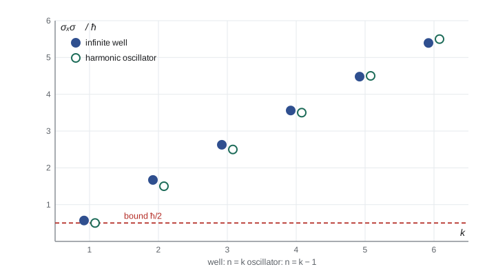
Uncertainty products for known states

For the oscillator, lesson 5 found \(\sigma_x\sigma_p = (n + \tfrac12)\hbar\). For the infinite well of width \(a\), \(\langle p^2\rangle = (n\pi\hbar/a)^2\) and \(\sigma_x^2 = a^2(1/12 - 1/2n^2\pi^2)\), so \(\sigma_x\sigma_p = \hbar\sqrt{n^2\pi^2/12 - 1/2}\), which for \(n = 1\) is \(0.568\hbar\): close to the bound, because the sine arch is nearly Gaussian, but not on it. The program below computes these products by numerical integration, then samples measurements of energy on a superposition state, showing that the results are always eigenvalues with the predicted frequencies.

import math, random
hbar = 1.0
def products_box(n, a=1.0, N=20000):
    dx = a / N; xs = [(i + 0.5) * dx for i in range(N)]
    psi = [math.sqrt(2 / a) * math.sin(n * math.pi * x / a) for x in xs]
    dpsi = [math.sqrt(2 / a) * (n * math.pi / a) * math.cos(n * math.pi * x / a) for x in xs]
    mx = sum(x * p * p for x, p in zip(xs, psi)) * dx
    vx = sum((x - mx) ** 2 * p * p for x, p in zip(xs, psi)) * dx
    p2 = hbar ** 2 * sum(d * d for d in dpsi) * dx          # <p^2> = hbar^2 int |psi'|^2
    return math.sqrt(vx * p2)
def products_osc(n, N=20000, L=12.0):
    dx = 2 * L / N; xs = [-L + (i + 0.5) * dx for i in range(N)]
    def H(k, x):
        h0, h1 = 1.0, 2 * x
        if k == 0: return h0
        for j in range(1, k): h0, h1 = h1, 2 * x * h1 - 2 * j * h0
        return h1
    c = 1 / math.sqrt(2 ** n * math.factorial(n) * math.sqrt(math.pi))
    psi = [c * H(n, x) * math.exp(-x * x / 2) for x in xs]
    dpsi = [(psi[i + 1] - psi[i - 1]) / (2 * dx) for i in range(1, N - 1)]
    vx = sum(x * x * p * p for x, p in zip(xs, psi)) * dx
    p2 = sum(d * d for d in dpsi) * dx
    return math.sqrt(vx * p2)
print(" n   box sigma_x sigma_p    formula      oscillator (n from 0)   n + 1/2")
for n in range(1, 7):
    f = math.sqrt(n * n * math.pi ** 2 / 12 - 0.5)
    print(f" {n}       {products_box(n):.4f}         {f:.4f}         {products_osc(n - 1):.4f}            {n - 0.5:.1f}")
# energy measurements on psi = (psi1 + 2 psi2 + 2i psi3)/3 in a box (E_n = n^2 in units of E1)
rnd = random.Random(372)
c = [1 / 3, 2 / 3, 2j / 3]
probs = [abs(z) ** 2 for z in c]
counts = [0, 0, 0]
for _ in range(9000):
    r, acc = rnd.random(), 0.0
    for k, p in enumerate(probs):
        acc += p
        if r < acc: counts[k] += 1; break
print("energy results (units of E1):", {1: counts[0], 4: counts[1], 9: counts[2]})
print("predicted fractions:", [round(p, 4) for p in probs], " observed:", [round(k / 9000, 4) for k in counts])
mean = sum(n * n * k for n, k in zip((1, 2, 3), counts)) / 9000
print(f"mean of results {mean:.3f}   <H> = sum |c_n|^2 E_n = {sum(p * n * n for p, n in zip(probs, (1, 2, 3))):.3f}")

 n   box sigma_x sigma_p    formula      oscillator (n from 0)   n + 1/2
 1       0.5679         0.5679         0.5000            0.5
 2       1.6703         1.6703         1.5000            1.5
 3       2.6272         2.6272         2.5000            2.5
 4       3.5580         3.5580         3.5000            3.5
 5       4.4790         4.4790         4.5000            4.5
 6       5.3953         5.3953         5.5000            5.5
energy results (units of E1): {1: 991, 4: 4015, 9: 3994}
predicted fractions: [0.1111, 0.4444, 0.4444]  observed: [0.1101, 0.4461, 0.4438]
mean of results 5.889   <H> = sum |c_n|^2 E_n = 5.889

Energy and time

Energy and time also obey an uncertainty relation, \(\Delta E\,\Delta t \geq \hbar/2\), but it has a different status, because time is not an observable with an operator; it is a parameter. The correct statement involves how fast things change. For any observable \(Q\), differentiating \(\langle Q\rangle\) and using the Schrödinger equation for both \(\Psi\) and \(\Psi^{*}\) gives the generalized Ehrenfest theorem

Applying the uncertainty principle to \(\hat H\) and a time-independent \(\hat Q\) gives \(\sigma_H\sigma_Q \geq \tfrac{\hbar}{2}|d\langle Q\rangle/dt|\). Define \(\Delta t = \sigma_Q/|d\langle Q\rangle/dt|\), the time it takes \(\langle Q\rangle\) to change by one standard deviation; then \(\Delta E\,\Delta t \geq \hbar/2\) with \(\Delta E = \sigma_H\). This is the Mandelstam–Tamm form, from 1945. A state with a sharp energy changes slowly; to change quickly, a state must be a superposition of widely different energies. A stationary state has \(\sigma_H = 0\), and indeed nothing about it changes. An excited atom that decays in a lifetime \(\tau\) has an energy spread of about \(\hbar/\tau\), seen as the natural width of its spectral line: for the 2p state of hydrogen, with \(\tau = 1.6\) ns, the width is about \(4 \times 10^{-7}\) eV.

Conservation laws

The generalized Ehrenfest theorem gives the quantum form of conservation laws. If \(\hat Q\) does not depend explicitly on time and commutes with \(\hat H\), then \(d\langle Q\rangle/dt = 0\) in every state. More than that, the probabilities of all its eigenvalues are constant, since commuting operators share eigenvectors and the Hamiltonian then multiplies each component by a phase. Energy is always conserved, because \(\hat H\) commutes with itself. Momentum is conserved when \(V\) is constant, because \([\hat H, \hat p] = [V, \hat p] = i\hbar V'\). Angular momentum is conserved for a spherically symmetric potential, lesson 11. Parity is conserved for a symmetric potential, which is why its eigenstates could be chosen even or odd. Each conservation law corresponds to a symmetry of the Hamiltonian, the quantum version of Noether's theorem from classical mechanics (PHYS-344).