The finite square well and scattering in one dimension

Real wells have walls of finite height. A particle in a finite well has a finite number of bound states, whose wave functions leak into the walls, and above the top of the well a continuum of scattering states, which can be reflected even though nothing classical would stop them. PHYS-271 found the bound states of one finite well numerically, by shooting. This lesson solves the problem analytically, reducing it to transcendental equations with a clear graphical meaning, and then develops the general machinery of one-dimensional scattering: reflection and transmission at steps, wells and barriers, the transfer-matrix method, and the resonances that make some structures perfectly transparent at special energies. Those resonances explain an old puzzle in atomic physics, the Ramsauer–Townsend effect, and a modern semiconductor device, the resonant tunnelling diode.

Bound states of the finite well

Let \(V = -V_0\) for \(|x| < a\) and \(V = 0\) outside, a well of depth \(V_0\) and width \(2a\) placed symmetrically about the origin. Look for bound states, \(-V_0 < E < 0\). Inside, \(\psi'' = -l^2\psi\) with \(l = \sqrt{2m(E + V_0)}/\hbar\), so the solutions oscillate as \(\sin lx\) and \(\cos lx\). Outside, \(\psi'' = \kappa^2\psi\) with \(\kappa = \sqrt{-2mE}/\hbar\), and normalizability keeps only \(e^{-\kappa x}\) for \(x > a\) and \(e^{\kappa x}\) for \(x < -a\). Because the potential is even, the solutions can be taken even or odd (lesson 3), and it is enough to match at \(x = a\).

For even solutions, \(\psi = D\cos lx\) inside and \(Fe^{-\kappa x}\) outside. Continuity of \(\psi\) and \(\psi'\) at \(x = a\) gives \(D\cos la = Fe^{-\kappa a}\) and \(-lD\sin la = -\kappa Fe^{-\kappa a}\). Dividing the second by the first eliminates the constants:

the odd condition following in the same way from \(\psi = D\sin lx\) inside. Both \(\kappa\) and \(l\) depend on \(E\), so these are equations for the allowed energies. Introduce the dimensionless variables \(z = la\) and \(z_0 = (a/\hbar)\sqrt{2mV_0}\), a single number that measures the strength of the well. Since \(\kappa^2 + l^2 = 2mV_0/\hbar^2\), we have \(\kappa a = \sqrt{z_0^2 - z^2}\), and the even condition becomes

This transcendental equation has no closed-form solution, but its graphical meaning is clear. Plot \(\tan z\) and the right side, which starts at infinity at \(z = 0\) and falls to zero at \(z = z_0\). Each branch of the tangent, starting at \(z = 0, \pi, 2\pi, \ldots\), crosses the falling curve once, provided the branch starts before \(z_0\). The odd states come from \(-\cot z\), whose branches start at \(\pi/2, 3\pi/2, \ldots\). Counting crossings gives the number of bound states: \(N = \lceil 2z_0/\pi \rceil\), the smallest integer at least \(2z_0/\pi\).

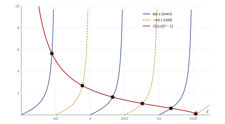
Two limits check the result. For a wide, deep well, \(z_0 \to \infty\), the crossings approach the asymptotes of the tangent, \(z \to n\pi/2\), so \(E + V_0 \to n^2\pi^2\hbar^2/2m(2a)^2\): the infinite-well energies for width \(2a\), measured from the bottom. For a shallow, narrow well, \(z_0 < \pi/2\), there is exactly one bound state, and no well in one dimension is too weak to bind one. In three dimensions that is false: a spherical well must be deep enough, which is why the deuteron, the only bound state of a neutron and a proton, is so weakly bound, at 2.22 MeV, and why the two-neutron system is not bound at all.

Every finite-well energy lies below the corresponding infinite-well energy for the same width. The wave function leaks into the walls, so it fits into an effectively wider region and needs less curvature. The program below finds the bound states of a well of depth 10 eV and width 0.6 nm for an electron by bisection on the transcendental equations, then compares them with the infinite well.

import math
hbar, me, eV = 1.054571817e-34, 9.1093837e-31, 1.602176634e-19
V0, a = 10.0 * eV, 0.3e-9                # depth and half-width
z0 = a * math.sqrt(2 * me * V0) / hbar
print(f"z0 = {z0:.4f};  number of bound states = ceil(2 z0 / pi) = {math.ceil(2 * z0 / math.pi)}")
def f_even(z): return math.tan(z) - math.sqrt((z0 / z) ** 2 - 1)
def f_odd(z):  return -1 / math.tan(z) - math.sqrt((z0 / z) ** 2 - 1)
def bisect(f, lo, hi):
    for _ in range(80):
        mid = 0.5 * (lo + hi)
        if f(lo) * f(mid) <= 0: hi = mid
        else: lo = mid
    return 0.5 * (lo + hi)
roots = []
n = 0
while n * math.pi / 2 < z0:
    lo = n * math.pi / 2 + 1e-9
    hi = min((n + 1) * math.pi / 2 - 1e-9, z0 - 1e-12)
    f = f_even if n % 2 == 0 else f_odd
    if f(lo) * f(hi) < 0: roots.append((n + 1, bisect(f, lo, hi), 'even' if n % 2 == 0 else 'odd'))
    n += 1
E_inf = lambda k: (k * math.pi * hbar) ** 2 / (2 * me * (2 * a) ** 2) / eV
print(" state  parity   z        E (eV)   E + V0   infinite well (width 2a)")
for k, z, par in roots:
    E = (hbar * z / a) ** 2 / (2 * me) / eV - 10.0
    print(f"  {k}     {par:4s}   {z:.4f}   {E:7.3f}   {E + 10:6.3f}       {E_inf(k):6.3f}")
k = roots[0][1] / a; kap = math.sqrt(z0 ** 2 - roots[0][1] ** 2) / a
print(f"ground state decay length outside: 1/kappa = {1e9 / kap:.4f} nm")

z0 = 4.8603;  number of bound states = ceil(2 z0 / pi) = 4
 state  parity   z        E (eV)   E + V0   infinite well (width 2a)
  1     even   1.3000    -9.285    0.715        1.045
  2     odd    2.5816    -7.179    2.821        4.178
  3     even   3.8111    -3.851    6.149        9.401
  4     odd    4.8279    -0.133    9.867       16.712
ground state decay length outside: 1/kappa = 0.0641 nm

Scattering: the general setup

Now consider a particle with \(E > 0\), coming in from the left toward a localized potential. On the far left the solution is \(Ae^{ikx} + Be^{-ikx}\), an incident and a reflected wave; on the far right it is \(Fe^{ik'x}\), the transmitted wave, where \(k\) and \(k'\) are the wave numbers on each side (different if the potential levels differ). As in lesson 6, the physical quantities are the probability currents, \(\hbar k|A|^2/m\) incident, \(\hbar k|B|^2/m\) reflected and \(\hbar k'|F|^2/m\) transmitted, so

The factor \(k'/k\) matters whenever the potential on the two sides differs. Take a potential step, \(V = 0\) for \(x < 0\) and \(V = V_0\) for \(x > 0\), with \(E > V_0\). Matching \(\psi\) and \(\psi'\) at zero gives \(F = 2kA/(k + k')\) and \(B = (k - k')A/(k + k')\), so

the same formulas as for light crossing a boundary between media of different refractive index, with wave number playing the role of index. A particle partly reflects from a step it has plenty of energy to climb, and, strikingly, it reflects just as much from a step down: the formula is symmetric in \(k\) and \(k'\). For \(E < V_0\), \(k'\) becomes imaginary, the transmitted wave decays, it carries no current, and \(R = 1\): total reflection, with an evanescent tail penetrating the step, the quantum counterpart of frustrated total internal reflection in optics.

Scattering over the finite well

For the finite well with \(E > 0\), the inside wave number is \(l = \sqrt{2m(E + V_0)}/\hbar\). Matching at both edges, four equations in \(A\), \(B\), \(F\) and the two inside amplitudes, gives after some algebra

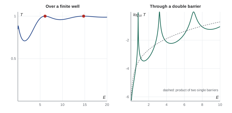
The well is perfectly transparent, \(T = 1\), whenever the sine vanishes, that is when \(2al = n\pi\): an integer number of half wavelengths fits across the well, so the waves reflected at the two edges cancel exactly, like the reflections from the two faces of an antireflection coating. Between these resonances some reflection occurs. Remarkably, the resonance energies \(E_n + V_0 = n^2\pi^2\hbar^2/2m(2a)^2\) are exactly the infinite-well energies. In 1921 Carl Ramsauer, and independently John Townsend and V. A. Bailey, found that slow electrons pass through argon and other noble-gas atoms almost without scattering at an energy near 1 eV, which no classical model could explain. The Ramsauer–Townsend effect is this resonance in three dimensions, the attractive atomic potential acting as a well whose size and depth make it transparent at that energy.

Transfer matrices

For any potential made of flat pieces, scattering can be computed systematically. In each region \(j\), with wave number \(k_j\), the solution is \(A_je^{ik_jx} + B_je^{-ik_jx}\). Matching \(\psi\) and \(\psi'\) at a boundary at \(x = d\) relates the amplitudes on the two sides by a 2 by 2 matrix, and the matrices for successive boundaries multiply. With the convention that the overall matrix \(M\) maps the right-hand amplitudes \((F, 0)\) to the left-hand ones \((A, B)\), the transmission is \(T = (k_{\mathrm{right}}/k_{\mathrm{left}})/|M_{11}|^2\). The method handles barriers (where \(k_j\) is imaginary) as easily as wells, and any number of layers. It is the same method used to design thin-film optical coatings, applied to matter waves.

Resonant tunnelling

Put two thin barriers a short distance apart. A particle with energy below the barrier tops would tunnel through each with small probability, and classically one would expect the probabilities to multiply. Instead, at energies where the region between the barriers would hold a quasi-bound state, the waves bouncing between the barriers add up in phase and the transmission rises to one, however opaque each barrier is on its own. Between resonances it is far smaller than for one barrier. Leo Esaki and Raphael Tsu proposed exploiting this in semiconductor layers in 1973, and the resonant tunnelling diode, built in 1974 by L. L. Chang, Esaki and Tsu, shows the sharp current peaks that result as the voltage sweeps the resonance through the energy of the incoming electrons. Esaki shared the 1973 Nobel Prize for discovering tunnelling in semiconductor junctions. The program below computes transmission through such a double barrier with transfer matrices and finds the resonances.

import cmath, math
hbar = m = 1.0
def transmission(E, layers):
    """layers: list of (V, width) between free regions with V = 0. Returns T."""
    regions = [(0.0, None)] + layers + [(0.0, None)]
    ks = [cmath.sqrt(2 * m * (E - V)) / hbar for V, _ in regions]
    M = [[1, 0], [0, 1]]
    x = 0.0
    for j in range(len(regions) - 1):
        k1, k2 = ks[j], ks[j + 1]
        # amplitudes (A1, B1) in region j from (A2, B2) in region j + 1 at boundary x
        r = k2 / k1
        e = lambda s: cmath.exp(1j * s * x)
        D = [[0.5 * (1 + r) * e(k2 - k1), 0.5 * (1 - r) * e(-k2 - k1)],
             [0.5 * (1 - r) * e(k2 + k1), 0.5 * (1 + r) * e(-k2 + k1)]]
        M = [[M[0][0] * D[0][0] + M[0][1] * D[1][0], M[0][0] * D[0][1] + M[0][1] * D[1][1]],
             [M[1][0] * D[0][0] + M[1][1] * D[1][0], M[1][0] * D[0][1] + M[1][1] * D[1][1]]]
        if regions[j + 1][1] is not None: x += regions[j + 1][1]
    return (ks[-1] / ks[0]).real / abs(M[0][0]) ** 2
V0, b, w = 10.0, 0.5, 2.0                 # barrier height, barrier width, gap
single = [(V0, b)]
double = [(V0, b), (0.0, w), (V0, b)]
print(f"single barrier at E = 1: T = {transmission(1.0, single):.4e}")
print(f"product of two single-barrier T: {transmission(1.0, single) ** 2:.4e}")
print(f"double barrier at E = 1: T = {transmission(1.0, double):.4e}")
# find resonances below the barrier top by scanning
Es = [0.005 * i for i in range(1, 2000)]
Ts = [transmission(E, double) for E in Es]
peaks = [Es[i] for i in range(1, len(Es) - 1) if Ts[i] > Ts[i - 1] and Ts[i] > Ts[i + 1] and Ts[i] > 0.01]
for nres, Ep in enumerate(peaks, 1):
    lo, hi = Ep - 0.005, Ep + 0.005       # refine by golden-section search
    for _ in range(60):
        m1, m2 = lo + 0.382 * (hi - lo), lo + 0.618 * (hi - lo)
        if transmission(m1, double) > transmission(m2, double): hi = m2
        else: lo = m1
    Er = 0.5 * (lo + hi)
    box = (nres * math.pi * hbar) ** 2 / (2 * m * w ** 2)
    print(f"resonance {nres} at E = {Er:.4f}: T = {transmission(Er, double):.6f}   (infinite well of width {w}: E{nres} = {box:.4f})")
# check R + T = 1 for a step-free case above the barriers
print(f"well with V0 = -5, width 2, at E = 2: T = {transmission(2.0, [(-5.0, 2.0)]):.6f}")
lw = math.sqrt(2 * (2.0 + 5.0))
print(f"formula: {1 / (1 + 25 / (4 * 2.0 * 7.0) * math.sin(2.0 * lw) ** 2):.6f}")

single barrier at E = 1: T = 2.0856e-02
product of two single-barrier T: 4.3496e-04
double barrier at E = 1: T = 9.7444e-04
resonance 1 at E = 0.8132: T = 1.000000   (infinite well of width 2.0: E1 = 1.2337)
resonance 2 at E = 3.2045: T = 1.000000   (infinite well of width 2.0: E2 = 4.9348)
resonance 3 at E = 7.0268: T = 1.000000   (infinite well of width 2.0: E3 = 11.1033)
well with V0 = -5, width 2, at E = 2: T = 0.720539
formula: 0.720539

At each resonance the double barrier transmits perfectly, although a single barrier alone passes only about one particle in fifty, and the pair off resonance passes fewer than one in a thousand. Each resonance lies below the corresponding level of an infinite well the width of the gap, because the wave function leaks into the barriers, the same effect that lowers finite-well bound states. The last two lines check the transfer-matrix code against the analytic formula for the finite well.