The quantum harmonic oscillator: algebraic and analytic methods

Almost every potential looks like a parabola near its minimum. Expanding \(V(x)\) about a stable equilibrium \(x_0\) gives \(V \approx V(x_0) + \tfrac12V''(x_0)(x - x_0)^2\), because the first derivative vanishes there. So small vibrations of any system, a diatomic molecule, an atom in a crystal, a trapped ion, a mode of the electromagnetic field, are governed by the harmonic oscillator. In quantum mechanics it is the most important exactly solvable problem after hydrogen, and it can be solved in two completely different ways. The algebraic method, using ladder operators, is elegant and generalizes to angular momentum (lesson 11) and to quantum field theory. The analytic method, a power series for the differential equation, shows where quantization comes from and introduces the Hermite polynomials. This lesson does both.

The problem

A particle of mass \(m\) in the potential \(V = \tfrac12m\omega^2x^2\) oscillates classically with angular frequency \(\omega\) at any amplitude. The quantum problem is the time-independent equation

Two scales are built from \(m\), \(\omega\) and \(\hbar\): an energy \(\hbar\omega\) and a length \(\sqrt{\hbar/m\omega}\). For a hydrogen chloride molecule vibrating at \(\omega = 5.45 \times 10^{14}\) per second, with reduced mass \(1.63 \times 10^{-27}\) kg, these are 0.36 eV and 0.011 nm: vibrational quanta are a few tenths of an electronvolt, absorbed in the infrared, and the zero-point motion is nearly a tenth of the bond length of 0.127 nm.

The algebraic method

Write the Hamiltonian as \(\hat H = (\hat p^2 + m^2\omega^2\hat x^2)/2m\). If \(\hat x\) and \(\hat p\) were numbers, we could factor the sum of squares as \((m\omega x - i p)(m\omega x + i p)\). They are operators that do not commute, so the factoring leaves a remainder. Define the ladder operators

The key fact is the canonical commutator. Acting on any test function \(f\), \([\hat x, \hat p]f = x(-i\hbar f') - (-i\hbar)(xf)' = i\hbar f\), so

Multiplying out \(\hat a_-\hat a_+\) gives \((\hat p^2 + m^2\omega^2\hat x^2)/2\hbar m\omega - (i/2\hbar)[\hat x, \hat p] = \hat H/\hbar\omega + \tfrac12\), and similarly \(\hat a_+\hat a_- = \hat H/\hbar\omega - \tfrac12\). Hence

Now the ladder property. Suppose \(\hat H\psi = E\psi\). Then

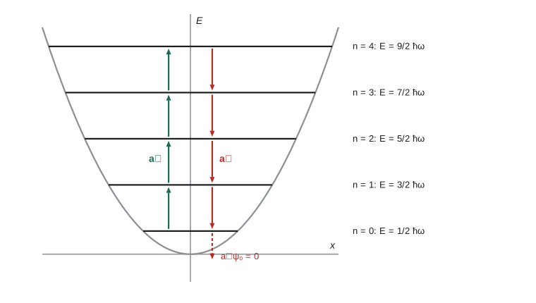
using \(\hat a_-\hat a_+ = \hat a_+\hat a_- + 1\). So \(\hat a_+\psi\) is an eigenfunction with energy one quantum higher, and in the same way \(\hat a_-\psi\) has energy \(E - \hbar\omega\). The operators climb up and down a ladder of levels spaced by \(\hbar\omega\). The ladder cannot go down forever, because the energy is bounded below (lesson 3: \(E > V_{\min} = 0\)). There must be a lowest rung \(\psi_0\) for which lowering gives zero, \(\hat a_-\psi_0 = 0\). That is a first-order differential equation:

The ground state is a Gaussian, and its energy follows from \(\hat H\psi_0 = \hbar\omega(\hat a_+\hat a_-\psi_0 + \tfrac12\psi_0) = \tfrac12\hbar\omega\,\psi_0\). Climbing the ladder gives every other state:

The factor \(1/\sqrt{n!}\) keeps the states normalized. To see why, note that \(\hat a_+\) and \(\hat a_-\) are Hermitian conjugates of each other, \(\int f^{*}(\hat a_{\pm}g)\,dx = \int(\hat a_{\mp}f)^{*}g\,dx\), which follows from integrating the derivative by parts. Then \(\int|\hat a_+\psi_n|^2dx = \int\psi_n^{*}\hat a_-\hat a_+\psi_n\,dx = n + 1\), so \(\hat a_+\psi_n = \sqrt{n + 1}\,\psi_{n+1}\), and likewise \(\hat a_-\psi_n = \sqrt n\,\psi_{n-1}\). The operator \(\hat N = \hat a_+\hat a_-\) counts the quanta, \(\hat N\psi_n = n\psi_n\). These are exactly the creation and annihilation operators of quantum field theory, where \(n\) counts photons in a mode of light or phonons in a crystal.

The analytic method

The same answer can be found by attacking the differential equation directly. In the dimensionless variable \(\xi = x\sqrt{m\omega/\hbar}\) and with \(K = 2E/\hbar\omega\), the equation becomes

For large \(\xi\) the \(K\) term is negligible and \(\psi \approx e^{\pm\xi^2/2}\); only the decaying sign is normalizable. So write \(\psi = h(\xi)e^{-\xi^2/2}\) and substitute, which gives Hermite's equation \(h'' - 2\xi h' + (K - 1)h = 0\). Try a power series \(h = \sum_j a_j\xi^j\). Collecting powers of \(\xi\) gives the recursion

Starting from \(a_0\) generates an even series and from \(a_1\) an odd one. Here is where quantization appears. For large \(j\) the recursion becomes \(a_{j+2} \approx (2/j)a_j\), the same as the series of \(e^{\xi^2}\). An infinite series would therefore grow like \(e^{\xi^2}\), and \(\psi = he^{-\xi^2/2}\) would blow up like \(e^{\xi^2/2}\). The only normalizable solutions are those for which the series stops: for some \(n\), the numerator \(2n + 1 - K\) must vanish, and the other series (odd if \(n\) is even, even if \(n\) is odd) must be absent. So \(K = 2n + 1\), which is \(E = (n + \tfrac12)\hbar\omega\) again. The terminating polynomials, normalized conventionally, are the Hermite polynomials \(H_n(\xi)\):

and the normalized eigenfunctions are

The analytic method shows clearly why energies are quantized. The Schrödinger equation has a solution for every energy, but for most energies the solution explodes at large \(|x|\). Only at special energies does it decay, and those are the levels. The same mechanism produces the hydrogen levels in lesson 12, through the termination of a different series.

Properties of the states

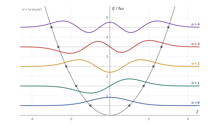
The eigenfunctions are alternately even and odd, since the potential is symmetric, and \(\psi_n\) has \(n\) nodes. They are orthonormal and complete, so any initial state can be expanded in them, and because the energies are equally spaced, \(E_n = (n + \tfrac12)\hbar\omega\), every state returns to its initial form, up to an overall phase, after one classical period \(2\pi/\omega\). The quantum oscillator, like the classical one, is perfectly periodic.

Expectation values are easy with ladder operators, since \(\hat x = \sqrt{\hbar/2m\omega}(\hat a_+ + \hat a_-)\) and \(\hat p = i\sqrt{\hbar m\omega/2}(\hat a_+ - \hat a_-)\). In any stationary state \(\langle x\rangle = \langle p\rangle = 0\), because \(\hat a_{\pm}\psi_n\) is orthogonal to \(\psi_n\). The squares give \(\langle x^2\rangle = (n + \tfrac12)\hbar/m\omega\) and \(\langle p^2\rangle = (n + \tfrac12)\hbar m\omega\), so the average potential and kinetic energies are equal, each \(\tfrac12E_n\), as in the classical virial theorem, and \(\sigma_x\sigma_p = (n + \tfrac12)\hbar\). The ground state is a minimum-uncertainty Gaussian, with \(\sigma_x\sigma_p = \hbar/2\).

Each eigenfunction extends beyond the classical turning points, where \(E_n = V\). For the ground state the turning points are at \(\xi = \pm1\), and the probability of finding the particle outside them is \(1 - \mathrm{erf}(1) = 0.157\): about one measurement in six finds the oscillator where a classical particle with the same energy could never be. At large \(n\), the probability density approaches the classical distribution, which is largest near the turning points, where the classical particle moves slowly, and smallest in the middle. The program below checks the energy levels and this forbidden-region probability.

import math
# Finite-difference oscillator in units hbar = m = omega = 1: H = -0.5 d2/dx2 + 0.5 x^2
L, N = 8.0, 800
dx = 2 * L / (N + 1)
xs = [-L + (j + 1) * dx for j in range(N)]
diag = [1 / dx ** 2 + 0.5 * x * x for x in xs]
off = -0.5 / dx ** 2
def count_below(E):                   # Sturm sequence: eigenvalues of a symmetric tridiagonal below E
    c, q = 0, 1.0
    for j in range(N):
        q = diag[j] - E - (off * off / q if j else 0.0)
        if q == 0: q = 1e-300
        if q < 0: c += 1
    return c
def eigen(k):                         # k-th eigenvalue (k = 0, 1, ...) by bisection
    lo, hi = 0.0, 20.0
    for _ in range(60):
        mid = 0.5 * (lo + hi)
        if count_below(mid) > k: hi = mid
        else: lo = mid
    return 0.5 * (lo + hi)
print(" n   finite-difference E_n   exact n + 1/2")
for n in range(6):
    print(f"{n:2d}       {eigen(n):.6f}           {n + 0.5:.1f}")
# Hermite polynomials by recursion, and the normalized eigenfunctions
def hermite(n, x):
    h0, h1 = 1.0, 2 * x
    if n == 0: return h0
    for k in range(1, n):
        h0, h1 = h1, 2 * x * h1 - 2 * k * h0
    return h1
def psi(n, x):
    return hermite(n, x) * math.exp(-x * x / 2) / math.sqrt(2 ** n * math.factorial(n) * math.sqrt(math.pi))
g = [-10 + 0.001 * i for i in range(20001)]
print("overlaps <psi_m|psi_n> for m, n in 0..3:")
for m_ in range(4):
    row = [sum(psi(m_, x) * psi(n, x) for x in g) * 0.001 for n in range(4)]
    print("  " + "  ".join(f"{(v if abs(v) > 5e-5 else 0.0): .4f}" for v in row))
for n in (0, 1, 5, 20):
    xt = math.sqrt(2 * n + 1)         # classical turning point
    out = sum(psi(n, x) ** 2 for x in g if abs(x) > xt) * 0.001
    print(f"n = {n:2d}: turning point {xt:.3f}, probability outside {out:.4f}")
print(f"ground state exact: 1 - erf(1) = {1 - math.erf(1):.4f}")

 n   finite-difference E_n   exact n + 1/2
 0       0.499988           0.5
 1       1.499938           1.5
 2       2.499838           2.5
 3       3.499688           3.5
 4       4.499489           4.5
 5       5.499239           5.5
overlaps <psi_m|psi_n> for m, n in 0..3:
   1.0000   0.0000   0.0000   0.0000
   0.0000   1.0000   0.0000   0.0000
   0.0000   0.0000   1.0000   0.0000
   0.0000   0.0000   0.0000   1.0000
n =  0: turning point 1.000, probability outside 0.1571
n =  1: turning point 1.732, probability outside 0.1115
n =  5: turning point 3.317, probability outside 0.0741
n = 20: turning point 6.403, probability outside 0.0483
ground state exact: 1 - erf(1) = 0.1573

The finite-difference energies match \(n + \tfrac12\) to about four decimal places, with errors growing slowly with \(n\) as the eigenfunctions wiggle more on the grid. The probability of being outside the turning points falls as \(n\) grows, roughly as \(n^{-1/3}\), but slowly; even the twentieth state is found in the classically forbidden region about one time in twenty.

Oscillators in nature

Molecular vibrations are the classic application. A diatomic molecule's vibrational levels are nearly evenly spaced, and infrared spectroscopy (CHEM-282) measures the spacing, which gives the bond stiffness. The zero-point energy \(\tfrac12\hbar\omega\) is real and measurable: it differs between isotopes, because \(\omega\) depends on mass, which shifts chemical reaction rates and equilibria, the basis of isotope effects used in geochemistry and in tracing water through the environment. In a crystal, the vibrations of the lattice are a set of coupled oscillators whose quanta, phonons, carry heat (PHYS-261 used them for heat capacity). In quantum optics, each mode of the electromagnetic field is an oscillator whose quanta are photons, and the zero-point fluctuations of the field produce measurable effects, among them the Casimir force between close metal plates and the Lamb shift of hydrogen levels. In ion traps and superconducting circuits, single oscillator modes are now controlled one quantum at a time.