Quantum mechanics in three dimensions: separation in spherical coordinates

Atoms, nuclei and molecules live in three dimensions, and so must quantum mechanics. Nothing in the formalism of lessons 8 and 9 changes: states are still vectors, observables Hermitian operators, and the Schrödinger equation still governs time evolution. What changes is the geometry. The kinetic energy involves the full Laplacian, and the symmetry of the potential decides which coordinates make the equation separable. Boxes and oscillators separate in Cartesian coordinates, and their extra dimensions bring degeneracy, several states with the same energy. Potentials that depend only on the distance from a fixed point, the case for every atom, separate in spherical coordinates into an angular part, the same for every such potential, and a radial part that looks like a one-dimensional problem with an extra centrifugal term. This lesson carries out that separation and solves the simplest radial problem, the infinite spherical well. Lesson 11 handles the angular part and lesson 12 the hydrogen atom.

The Schrödinger equation in three dimensions

With momentum operator \(\hat{\mathbf p} = -i\hbar\nabla\), the kinetic energy becomes \(\hat{\mathbf p}^2/2m = -(\hbar^2/2m)\nabla^2\), and the time-dependent and time-independent equations are

The wave function \(\Psi(\mathbf r, t)\) gives the probability density \(|\Psi|^2\) per unit volume, normalized by \(\int|\Psi|^2\,d^3r = 1\). The canonical commutators generalize to \([\hat r_i, \hat p_j] = i\hbar\,\delta_{ij}\): each coordinate fails to commute with its own momentum component but commutes with the others. The probability current becomes a vector, \(\mathbf j = (\hbar/m)\,\mathrm{Im}(\Psi^{*}\nabla\Psi)\), obeying \(\partial_t|\Psi|^2 + \nabla\cdot\mathbf j = 0\). Stationary states, expansions in eigenfunctions and the uncertainty principle carry over unchanged.

Cartesian separation and degeneracy

In a rectangular box with sides \(a\), \(b\), \(c\) and infinite walls, try \(\psi = X(x)Y(y)Z(z)\). Dividing by \(XYZ\) splits the equation into three one-dimensional wells, each solved in lesson 4, and

For a cube, \(a = b = c\), the energy depends only on \(n_x^2 + n_y^2 + n_z^2\), and different triples with the same sum give the same energy. The ground state \((1,1,1)\) is unique, but the first excited level, \((2,1,1)\), \((1,2,1)\) and \((1,1,2)\), is threefold degenerate. Degeneracy is the rule in three dimensions, and it almost always reflects a symmetry: here, the equivalence of the three axes. Squash the cube slightly and the threefold level splits. Some degeneracies are accidental, arising from coincidences such as \(3^2 + 3^2 + 3^2 = 5^2 + 1^2 + 1^2 = 27\), where \((3,3,3)\) shares its energy with the three permutations of \((5,1,1)\).

The isotropic oscillator, \(V = \tfrac12m\omega^2r^2\), also separates in Cartesian coordinates into three oscillators of lesson 5, so \(E = (n_x + n_y + n_z + \tfrac32)\hbar\omega = (n + \tfrac32)\hbar\omega\). The number of ways to write \(n\) as a sum of three nonnegative integers is \((n + 1)(n + 2)/2\), so the levels have degeneracies 1, 3, 6, 10, and so on. This degeneracy pattern explains the first magic numbers of nuclear physics, 2, 8 and 20, where nuclei with filled oscillator shells are unusually stable, as Maria Goeppert Mayer and Hans Jensen showed in 1949 once the spin–orbit force was added for the higher ones.

Spherical coordinates

For a central potential \(V(r)\), the natural coordinates are \(r\), the polar angle \(\theta\) and the azimuth \(\phi\). The Laplacian becomes

and the volume element is \(d^3r = r^2\sin\theta\,dr\,d\theta\,d\phi\). Try \(\psi = R(r)\,Y(\theta, \phi)\). Substituting into the Schrödinger equation, multiplying by \(-2mr^2/\hbar^2RY\) and collecting terms puts everything depending on \(r\) on one side and everything depending on the angles on the other. Each side must then equal a constant, which for reasons that will become clear we write as \(l(l + 1)\):

The angular equation contains no trace of the potential. Its solutions, the spherical harmonics \(Y_l^m(\theta, \phi)\), are therefore the same for every central potential: hydrogen, the spherical well, the isotropic oscillator and the nucleus all share them. Lesson 11 shows that the angular equation is the eigenvalue equation for the square of the angular momentum, \(\hat L^2Y = \hbar^2l(l + 1)Y\), that single-valued, finite solutions exist only for \(l = 0, 1, 2, \ldots\), and that for each \(l\) there are \(2l + 1\) of them, labelled by \(m = -l, \ldots, l\).

The radial equation

The radial equation simplifies with the substitution \(u(r) = rR(r)\). Since \(\frac{d}{dr}(r^2R') = ru''\), it becomes

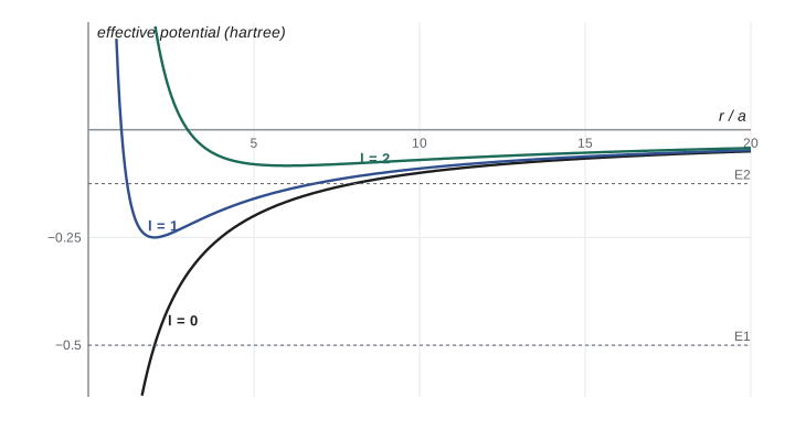
This is exactly the one-dimensional Schrödinger equation on the half-line \(r > 0\), with an effective potential

The extra term is the centrifugal barrier. Classically, a particle with angular momentum \(L\) has rotational kinetic energy \(L^2/2mr^2\), which grows as it approaches the origin and pushes it outward; the quantum version replaces \(L^2\) with \(\hbar^2l(l + 1)\). Normalization becomes \(\int_0^\infty|u|^2dr = 1\), because \(\int|R|^2r^2dr = \int|u|^2dr\) and the spherical harmonics are normalized on their own. And \(u(0) = 0\): otherwise \(R = u/r\) would blow up at the origin as \(1/r\), and \(\nabla^2(1/r)\) is a delta function that the potential cannot match. So every radial problem is a one-dimensional problem with a hard wall at \(r = 0\), and all the methods of lessons 3 to 7 apply. Near the origin, where the centrifugal term dominates, \(u \propto r^{l+1}\): states with higher \(l\) are pushed away from the origin, which in atoms determines which electrons screen which, and so the order in which subshells fill.

The infinite spherical well

As a first radial problem, take \(V = 0\) for \(r < a\) and \(V = \infty\) outside, a model of a particle confined in a cavity, a quark in a nucleon in the bag model, or a nucleon in a nucleus. For \(l = 0\) the radial equation is \(u'' = -k^2u\) with \(u(0) = u(a) = 0\), exactly the one-dimensional well: \(u = \sin(n\pi r/a)\) and \(E_{n0} = n^2\pi^2\hbar^2/2ma^2\). For general \(l\), the solutions that are finite at the origin are spherical Bessel functions, \(R = j_l(kr)\), with

The boundary condition \(j_l(ka) = 0\) quantizes the energy: if \(\beta_{nl}\) is the \(n\)th zero of \(j_l\), then \(E_{nl} = \hbar^2\beta_{nl}^2/2ma^2\). The zeros of \(j_0\) are \(\pi, 2\pi, 3\pi, \ldots\); those of \(j_1\) begin at 4.493 and of \(j_2\) at 5.763. So the levels in order are \(1s\) (\(\beta = 3.142\)), \(1p\) (4.493), \(1d\) (5.763), \(2s\) (6.283), \(1f\) (6.988), and so on, each with degeneracy \(2l + 1\) from the allowed values of \(m\). Unlike the oscillator, the spherical well has no degeneracy between different \(l\): the ordering of shells depends on the shape of the potential, which is how nuclear and atomic shell structures differ.

The program below finds the spherical-well energies two ways: from zeros of the spherical Bessel functions, found by bisection, and by solving the radial equation on a grid with the effective potential, using the Sturm-sequence eigenvalue method of lesson 5. It also counts the degeneracies of the cubic box.

import math
# degeneracies of the cubic box: energy in units of pi^2 hbar^2 / (2 m a^2) is nx^2 + ny^2 + nz^2
from collections import Counter
levels = Counter(nx * nx + ny * ny + nz * nz for nx in range(1, 7) for ny in range(1, 7) for nz in range(1, 7))
print("cubic box, lowest levels (n^2 sum: degeneracy):", [(s, levels[s]) for s in sorted(levels)[:8]])
print("accidental degeneracy at 27:", levels[27], "states, from (3,3,3) and permutations of (5,1,1)")
# spherical Bessel functions by upward recursion and their zeros
def jl(l, x):
    j0, j1 = math.sin(x) / x, math.sin(x) / x ** 2 - math.cos(x) / x
    if l == 0: return j0
    for k in range(1, l): j0, j1 = j1, (2 * k + 1) / x * j1 - j0
    return j1
def zeros(l, count):
    out, x, step = [], 0.5, 0.01
    while len(out) < count:
        if jl(l, x) * jl(l, x + step) < 0:
            lo, hi = x, x + step
            for _ in range(60):
                mid = 0.5 * (lo + hi)
                if jl(l, lo) * jl(l, mid) <= 0: hi = mid
                else: lo = mid
            out.append(0.5 * (lo + hi))
        x += step
    return out
# radial equation on a grid: -u''/2 + l(l+1)/(2 r^2) u = E u on 0 < r < 1 (hbar = m = a = 1), u(0) = u(1) = 0
N = 2000; h = 1.0 / (N + 1)
def eigen(l, k):
    d = [1 / h ** 2 + l * (l + 1) / (2 * ((j + 1) * h) ** 2) for j in range(N)]
    o2 = (0.5 / h ** 2) ** 2
    def count(E):
        c, q = 0, 1.0
        for j in range(N):
            q = d[j] - E - (o2 / q if j else 0.0)
            if q == 0: q = 1e-300
            if q < 0: c += 1
        return c
    lo, hi = 0.0, 400.0
    for _ in range(50):
        mid = 0.5 * (lo + hi)
        if count(mid) > k: hi = mid
        else: lo = mid
    return 0.5 * (lo + hi)
print(" level  l   Bessel zero   E = zero^2/2   grid E      degeneracy 2l+1")
rows = []
for l in range(4):
    for n, z in enumerate(zeros(l, 2), 1):
        rows.append((z, n, l))
for z, n, l in sorted(rows)[:6]:
    print(f"  {n}{'spdf'[l]}    {l}    {z:8.4f}     {z * z / 2:8.4f}    {eigen(l, n - 1):8.4f}       {2 * l + 1}")

cubic box, lowest levels (n^2 sum: degeneracy): [(3, 1), (6, 3), (9, 3), (11, 3), (12, 1), (14, 6), (17, 3), (18, 3)]
accidental degeneracy at 27: 4 states, from (3,3,3) and permutations of (5,1,1)
 level  l   Bessel zero   E = zero^2/2   grid E      degeneracy 2l+1
  1s    0      3.1416       4.9348      4.9348       1
  1p    1      4.4934      10.0954     10.0954       3
  1d    2      5.7635      16.6087     16.6087       5
  2s    0      6.2832      19.7392     19.7392       1
  1f    3      6.9879      24.4156     24.4156       7
  2p    1      7.7253      29.8398     29.8397       3

The grid solution of the radial equation agrees with the Bessel zeros to five or six significant figures, confirming that the effective potential correctly captures the angular motion. The degeneracy column counts only the \(2l + 1\) values of \(m\); with spin, each level holds twice as many fermions.

Where the angular momentum lives

The separation constant \(l(l + 1)\) is the first appearance of the quantum theory of angular momentum, which lesson 11 develops. It is worth seeing already why it must take this form. Classically, the energy of a particle in a central potential splits into radial kinetic energy plus \(L^2/2mr^2\). The angular part of the Laplacian, the operator in square brackets in the angular equation, is \(-\hat L^2/\hbar^2\), so the separated equation says \(\hat L^2Y = \hbar^2l(l + 1)Y\). The total angular momentum is quantized, with magnitude \(\hbar\sqrt{l(l + 1)}\), never exactly \(\hbar l\), and that subtle difference is one of the measurable predictions the old quantum theory of Bohr and Sommerfeld got wrong.